Я написал уникальный, не имеющий аналогов в мире однослойный персептрон без использования сторонних модулей. Для чего? Что бы всем показывать свою статью на Хабрахабре, очевидно же. Это не перевод и не копия чьей-нибудь статьи, всё своё.
Итак, весь код:
import random

def train(X, y, syn0, lens0, lens01, lr):
    errorreturn = 0
    for i in range(0, lens0):
        a = 0
        for j in range(0, lens01):
            a = a + syn0[i][j] * X[j]
        b = 1 / (1 + 2.718281828459045235360287471352662497757 ** -a)
        error = y[i] - b
        errorreturn = errorreturn + abs(error)
        delta = (error) * 1 / (1 + 2.718281828459045235360287471352662497757 ** -b) * lr
        for z in range(0, lens01):
            syn0[i][z] = syn0[i][z] + X[z] * delta
    return syn0, errorreturn

def predict(syn0, X, lens0, lens01):
    ret = []
    for i in range(0, lens0):
        a = 0
        for j in range(0, lens01):
            a = a + syn0[i][j] * X[j]
        b = 1 / (1 + 2.718281828459045235360287471352662497757 ** -a)
        ret.append(b)
    return ret

def trainmass(X, y, syn, lens0, lens01, lr, iter):
    for i in range(iter):
        for j in range(lens01):
            syn, er = train(X[j], y[j], syn, lens0, lens01, lr)
    return syn, er

def create(x, y):
    syn0 = []
    for z in range(0, x):
        h = []
        for i in range(0, y):
            h.append(random.uniform(-0.1, 0.1))
        syn0.append(h)
    return syn0

syn = create(2, 4)
X = [[0.1, 0.2, 0.3, 0.4],[0.2, 0.3, 0.4, 0.5],[0.4, 0.5, 0.6, 0.7],[0.5,0.6,0.7,0.8]]
y = [[0.5, 0.6],[0.6, 0.7],[0.8, 0.9],[0.9, 1]]
g, r = trainmass(X, y, syn, 2, 4, 1, 60000)
h = predict(syn, X[0], 2, 4)
h2 = predict(syn, [0.5, 0.6, 0.7, 0.8], 2, 4)
print(h)
print(h2)
Функция train — обучает, predict — обрабатывает входные данные уже обученными синапсами и выдает ответ, trainmass — запускает обучение по всем входным данным(2 — это количество выходных данных, 4 — количество данных в примере, 1 — это лерн рейт, 60000 — количество циклов обучения), create — создает массив случайных синапсов для обучения.
В этом примере массив X имеет 4 набора данных и массив y 4 набора выходных данных.
После запуска имеем вывод:
[0.4835439912709079, 0.5593653075469635]
[0.8848108739666853, 0.9682956213528969]
Первый массив — это ответ на входные данные X[0] — [0.1, 0.2, 0.3, 0.4].
Второй массив — это ответ на данные которые не были в обучающей выборке [0.5, 0.6, 0.7, 0.8].
Как видите персептрон продолжил числовой ряд почти верно с небольшими отклонениями.
Немного разберем принцип его работы. Персептрон получает что-то похожее на систему линейных уравнений:
0.1*x1 + 0.2*x2 + 0.3*x3 + 0.4*x4 = 0.5
0.2*x1 + 0.3*x2 + 0.4*x3 + 0.5*x4 = 0.6
0.4*x1 + 0.5*x2 + 0.6*x3 + 0.7*x4 = 0.8
0.5*x1 + 0.6*x2 + 0.7*x3 + 0.8*x4 = 0.9
И методом обратного распространения ошибки находит соответствующие x1, x2, x3, x4.
Для второго выходного значения создаются другие y1, y2, y3, y4.
Я не стану описывать функцию активации — сигмоид. Если вы разберетесь в этом простом коде вам станет понятно.
Однослойный персептрон может решать только линейные задачи. Для нелинейности нужно добавить еще слой или несколько слоев. Если будет много комментариев, я напишу двухслойную модель.
Перевод
Ссылка на автора
Алгоритм Perceptron — это самый простой тип искусственной нейронной сети.
Это модель одного нейрона, которая может использоваться для задач классификации двух классов и обеспечивает основу для дальнейшей разработки гораздо более крупных сетей.
В этом руководстве вы узнаете, как реализовать алгоритм Perceptron с нуля с помощью Python.
После завершения этого урока вы узнаете:
- Как тренировать сетевые веса для Перцептрона.
- Как делать прогнозы с помощью Перцептрона.
- Как реализовать алгоритм Персептрон для реальной задачи классификации.
Давайте начнем.
- Обновление январь / 2017: Изменено вычисление fold_size в cross_validation_split (), чтобы оно всегда было целым числом. Исправляет проблемы с Python 3.
- Обновление Авг / 2018: Протестировано и обновлено для работы с Python 3.6.

Описание
В этом разделе дается краткое введение в алгоритм Perceptron и набор данных Sonar, к которым мы позже применим его.
Алгоритм персептрона
Перцептрон вдохновлен обработкой информации одной нервной клетки, называемой нейроном.
Нейрон принимает входные сигналы через свои дендриты, которые передают электрический сигнал в тело клетки.
Аналогичным образом, Perceptron получает входные сигналы от примеров тренировочных данных, которые мы взвешиваем и объединяем в линейное уравнение, называемое активацией.
activation = sum(weight_i * x_i) + biasЗатем активация преобразуется в выходное значение или прогноз с использованием передаточной функции, такой как пошаговая передаточная функция.
prediction = 1.0 if activation >= 0.0 else 0.0Таким образом, Перцептрон является алгоритмом классификации для задач с двумя классами (0 и 1), где линейное уравнение (например, или гиперплоскость) может использоваться для разделения двух классов.
Это тесно связано с линейной регрессией и логистической регрессией, которые делают предсказания аналогичным образом (например, взвешенная сумма входных данных).
Вес алгоритма Perceptron должен быть оценен на основе ваших тренировочных данных с использованием стохастического градиентного спуска.
Стохастический градиентный спуск
Градиентный спуск — это процесс минимизации функции, следуя градиентам функции стоимости.
Это включает в себя знание формы стоимости, а также производной, чтобы из заданной точки вы знали градиент и могли двигаться в этом направлении, например, вниз к минимальному значению.
В машинном обучении мы можем использовать технику, которая оценивает и обновляет веса на каждой итерации, называемую стохастическим градиентным спуском, чтобы минимизировать ошибку модели в наших обучающих данных.
Этот алгоритм оптимизации работает так, что каждый обучающий экземпляр показывается модели по одному. Модель делает прогноз для обучающего экземпляра, вычисляется ошибка, и модель обновляется, чтобы уменьшить ошибку для следующего прогнозирования.
Эта процедура может использоваться, чтобы найти набор весов в модели, который приводит к наименьшей ошибке для модели в данных обучения.
Для алгоритма Perceptron каждая итерация весов (вес) обновляются с использованием уравнения:
w = w + learning_rate * (expected - predicted) * xкудавесвес оптимизируется,learning_rateэто скорость обучения, которую вы должны настроить (например, 0,01),(ожидается — предсказано)ошибка прогноза для модели на тренировочных данных, отнесенных к весу иИксэто входное значение.
Сонар Набор данных
Набор данных, который мы будем использовать в этом уроке, — это набор данных Sonar.
Это набор данных, который описывает возврат эхолота, отраженный от разных служб. 60 входных переменных — это сила отдачи под разными углами. Это проблема бинарной классификации, которая требует модели для дифференциации горных пород от металлических цилиндров.
Это хорошо понятный набор данных. Все переменные являются непрерывными и обычно находятся в диапазоне от 0 до 1. Таким образом, нам не нужно будет нормализовать входные данные, что часто является хорошей практикой в алгоритме Perceptron. Выходная переменная — это строка «M» для моего и «R» для рока, которую необходимо преобразовать в целые числа 1 и 0.
Прогнозируя класс с наибольшим количеством наблюдений в наборе данных (M или мин), алгоритм нулевого правила может достичь точности 53%.
Вы можете узнать больше об этом наборе данных на UCI хранилище машинного обучения, Вы можете скачать набор данных бесплатно и поместить его в свой рабочий каталог с именем файлаsonar.all-data.csv,
Руководство
Этот урок разбит на 3 части:
- Делать прогнозы.
- Весы тренировочные сети.
- Моделирование набора данных сонара.
Эти шаги дадут вам основу для реализации и применения алгоритма Perceptron к вашим собственным задачам прогнозного моделирования классификации.
1. Делать прогнозы
Первым шагом является разработка функции, которая может делать прогнозы.
Это будет необходимо как при оценке значений весов кандидатов при стохастическом градиентном спуске, так и после того, как модель будет завершена, и мы хотим начать делать прогнозы на тестовых данных или новых данных.
Ниже приведена функция с именемпредсказать, ()это предсказывает выходное значение для строки, заданной набором весов.
Первый вес всегда является смещением, поскольку он является автономным и не отвечает за конкретное входное значение.
# Make a prediction with weights
def predict(row, weights):
	activation = weights[0]
	for i in range(len(row)-1):
		activation += weights[i + 1] * row[i]
	return 1.0 if activation >= 0.0 else 0.0
Мы можем создать небольшой набор данных для проверки нашей функции прогнозирования.
X1			X2			Y
2.7810836		2.550537003		0
1.465489372		2.362125076		0
3.396561688		4.400293529		0
1.38807019		1.850220317		0
3.06407232		3.005305973		0
7.627531214		2.759262235		1
5.332441248		2.088626775		1
6.922596716		1.77106367		1
8.675418651		-0.242068655		1
7.673756466		3.508563011		1
Мы также можем использовать предварительно подготовленные веса, чтобы делать прогнозы для этого набора данных.
Собрав все это вместе, мы можем проверить нашипредсказать, ()функция ниже.
# Make a prediction with weights
def predict(row, weights):
	activation = weights[0]
	for i in range(len(row)-1):
		activation += weights[i + 1] * row[i]
	return 1.0 if activation >= 0.0 else 0.0

# test predictions
dataset = [[2.7810836,2.550537003,0],
	[1.465489372,2.362125076,0],
	[3.396561688,4.400293529,0],
	[1.38807019,1.850220317,0],
	[3.06407232,3.005305973,0],
	[7.627531214,2.759262235,1],
	[5.332441248,2.088626775,1],
	[6.922596716,1.77106367,1],
	[8.675418651,-0.242068655,1],
	[7.673756466,3.508563011,1]]
weights = [-0.1, 0.20653640140000007, -0.23418117710000003]
for row in dataset:
	prediction = predict(row, weights)
	print("Expected=%d, Predicted=%d" % (row[-1], prediction))
Есть два входных значения (X1а такжеX2) и три значения веса (смещение,w1а такжеw2). Уравнение активации, которое мы смоделировали для этой задачи:
activation = (w1 * X1) + (w2 * X2) + biasИли с конкретными значениями веса, которые мы выбрали вручную, как:
activation = (0.206 * X1) + (-0.234 * X2) + -0.1Запустив эту функцию, мы получим прогнозы, которые соответствуют ожидаемому результату (Y) ценности.
Expected=0, Predicted=0
Expected=0, Predicted=0
Expected=0, Predicted=0
Expected=0, Predicted=0
Expected=0, Predicted=0
Expected=1, Predicted=1
Expected=1, Predicted=1
Expected=1, Predicted=1
Expected=1, Predicted=1
Expected=1, Predicted=1
Теперь мы готовы реализовать стохастический градиентный спуск, чтобы оптимизировать наши значения веса.
2. Веса тренировочной сети
Мы можем оценить значения веса для наших тренировочных данных, используя стохастический градиентный спуск.
Стохастический градиентный спуск требует двух параметров:
- Скорость обучения: Используется для ограничения количества, которое корректируется каждый вес при каждом обновлении.
- Эпохи: Сколько раз пробегать данные тренировки при обновлении веса.
Они вместе с данными обучения будут аргументами функции.
В функции нам нужно выполнить 3 цикла:
- Зацикливайтесь на каждой эпохе.
- Зацикливайтесь на каждой строке в данных тренировки для определенной эпохи.
- Переберите каждый вес и обновите его для ряда в эпоху.
Как видите, мы обновляем каждый вес для каждой строки в тренировочных данных, каждую эпоху.
Веса обновляются в зависимости от ошибки, допущенной моделью. Ошибка рассчитывается как разница между ожидаемым выходным значением и прогнозом, сделанным с использованием весов-кандидатов.
Существует один вес для каждого входного атрибута, и они обновляются согласованным образом, например:
w(t+1)= w(t) + learning_rate * (expected(t) - predicted(t)) * x(t)Смещение обновляется аналогичным образом, за исключением того, что без ввода, поскольку оно не связано с конкретным значением ввода:
bias(t+1) = bias(t) + learning_rate * (expected(t) - predicted(t))Теперь мы можем собрать все это вместе. Ниже приведена функция с именемtrain_weights ()который вычисляет значения веса для учебного набора данных с использованием стохастического градиентного спуска.
# Estimate Perceptron weights using stochastic gradient descent
def train_weights(train, l_rate, n_epoch):
	weights = [0.0 for i in range(len(train[0]))]
	for epoch in range(n_epoch):
		sum_error = 0.0
		for row in train:
			prediction = predict(row, weights)
			error = row[-1] - prediction
			sum_error += error**2
			weights[0] = weights[0] + l_rate * error
			for i in range(len(row)-1):
				weights[i + 1] = weights[i + 1] + l_rate * error * row[i]
		print('>epoch=%d, lrate=%.3f, error=%.3f' % (epoch, l_rate, sum_error))
	return weights
Вы можете видеть, что мы также отслеживаем сумму квадратов ошибок (положительное значение) для каждой эпохи, чтобы мы могли распечатать хорошее сообщение в каждом внешнем цикле.
Мы можем протестировать эту функцию на том же небольшом измышленном наборе данных сверху.
# Make a prediction with weights
def predict(row, weights):
	activation = weights[0]
	for i in range(len(row)-1):
		activation += weights[i + 1] * row[i]
	return 1.0 if activation >= 0.0 else 0.0

# Estimate Perceptron weights using stochastic gradient descent
def train_weights(train, l_rate, n_epoch):
	weights = [0.0 for i in range(len(train[0]))]
	for epoch in range(n_epoch):
		sum_error = 0.0
		for row in train:
			prediction = predict(row, weights)
			error = row[-1] - prediction
			sum_error += error**2
			weights[0] = weights[0] + l_rate * error
			for i in range(len(row)-1):
				weights[i + 1] = weights[i + 1] + l_rate * error * row[i]
		print('>epoch=%d, lrate=%.3f, error=%.3f' % (epoch, l_rate, sum_error))
	return weights

# Calculate weights
dataset = [[2.7810836,2.550537003,0],
	[1.465489372,2.362125076,0],
	[3.396561688,4.400293529,0],
	[1.38807019,1.850220317,0],
	[3.06407232,3.005305973,0],
	[7.627531214,2.759262235,1],
	[5.332441248,2.088626775,1],
	[6.922596716,1.77106367,1],
	[8.675418651,-0.242068655,1],
	[7.673756466,3.508563011,1]]
l_rate = 0.1
n_epoch = 5
weights = train_weights(dataset, l_rate, n_epoch)
print(weights)
Мы используем скорость обучения 0,1 и обучаем модель только для 5 эпох, или 5 воздействий весов на весь набор обучающих данных.
При выполнении примера в каждую эпоху печатается сообщение с ошибкой суммы квадратов для этой эпохи и окончательным набором весов.
>epoch=0, lrate=0.100, error=2.000
>epoch=1, lrate=0.100, error=1.000
>epoch=2, lrate=0.100, error=0.000
>epoch=3, lrate=0.100, error=0.000
>epoch=4, lrate=0.100, error=0.000
[-0.1, 0.20653640140000007, -0.23418117710000003]
Вы можете увидеть, как алгоритм очень быстро изучает проблему.
Теперь давайте применим этот алгоритм к реальному набору данных.
3. Моделирование набора данных сонара
В этом разделе мы обучим модель персептрона с использованием стохастического градиентного спуска на наборе данных сонара.
В этом примере предполагается, что CSV-копия набора данных находится в текущем рабочем каталоге с именем файла.sonar.all-data.csv,
Сначала загружается набор данных, строковые значения преобразуются в числовые, а выходной столбец преобразуется из строк в целочисленные значения от 0 до 1. Это достигается с помощью вспомогательных функций.load_csv (),str_column_to_float ()а такжеstr_column_to_int ()загрузить и подготовить набор данных.
Мы будем использовать перекрестную проверку в k-кратном размере для оценки эффективности изученной модели на невидимых данных. Это означает, что мы будем строить и оценивать k моделей и оценивать производительность как среднюю ошибку модели. Точность классификации будет использоваться для оценки каждой модели. Эти поведения представлены вcross_validation_split (),accuracy_metric ()а такжеevaluate_algorithm ()вспомогательные функции.
Мы будем использоватьпрогнозировать () иtrain_weights ()функции, созданные выше, чтобы обучить модель и новыйперсептрон ()функция, чтобы связать их вместе.
Ниже приведен полный пример.
# Perceptron Algorithm on the Sonar Dataset
from random import seed
from random import randrange
from csv import reader

# Load a CSV file
def load_csv(filename):
	dataset = list()
	with open(filename, 'r') as file:
		csv_reader = reader(file)
		for row in csv_reader:
			if not row:
				continue
			dataset.append(row)
	return dataset

# Convert string column to float
def str_column_to_float(dataset, column):
	for row in dataset:
		row[column] = float(row[column].strip())

# Convert string column to integer
def str_column_to_int(dataset, column):
	class_values = [row[column] for row in dataset]
	unique = set(class_values)
	lookup = dict()
	for i, value in enumerate(unique):
		lookup[value] = i
	for row in dataset:
		row[column] = lookup[row[column]]
	return lookup

# Split a dataset into k folds
def cross_validation_split(dataset, n_folds):
	dataset_split = list()
	dataset_copy = list(dataset)
	fold_size = int(len(dataset) / n_folds)
	for i in range(n_folds):
		fold = list()
		while len(fold) < fold_size:
			index = randrange(len(dataset_copy))
			fold.append(dataset_copy.pop(index))
		dataset_split.append(fold)
	return dataset_split

# Calculate accuracy percentage
def accuracy_metric(actual, predicted):
	correct = 0
	for i in range(len(actual)):
		if actual[i] == predicted[i]:
			correct += 1
	return correct / float(len(actual)) * 100.0

# Evaluate an algorithm using a cross validation split
def evaluate_algorithm(dataset, algorithm, n_folds, *args):
	folds = cross_validation_split(dataset, n_folds)
	scores = list()
	for fold in folds:
		train_set = list(folds)
		train_set.remove(fold)
		train_set = sum(train_set, [])
		test_set = list()
		for row in fold:
			row_copy = list(row)
			test_set.append(row_copy)
			row_copy[-1] = None
		predicted = algorithm(train_set, test_set, *args)
		actual = [row[-1] for row in fold]
		accuracy = accuracy_metric(actual, predicted)
		scores.append(accuracy)
	return scores

# Make a prediction with weights
def predict(row, weights):
	activation = weights[0]
	for i in range(len(row)-1):
		activation += weights[i + 1] * row[i]
	return 1.0 if activation >= 0.0 else 0.0

# Estimate Perceptron weights using stochastic gradient descent
def train_weights(train, l_rate, n_epoch):
	weights = [0.0 for i in range(len(train[0]))]
	for epoch in range(n_epoch):
		for row in train:
			prediction = predict(row, weights)
			error = row[-1] - prediction
			weights[0] = weights[0] + l_rate * error
			for i in range(len(row)-1):
				weights[i + 1] = weights[i + 1] + l_rate * error * row[i]
	return weights

# Perceptron Algorithm With Stochastic Gradient Descent
def perceptron(train, test, l_rate, n_epoch):
	predictions = list()
	weights = train_weights(train, l_rate, n_epoch)
	for row in test:
		prediction = predict(row, weights)
		predictions.append(prediction)
	return(predictions)

# Test the Perceptron algorithm on the sonar dataset
seed(1)
# load and prepare data
filename = 'sonar.all-data.csv'
dataset = load_csv(filename)
for i in range(len(dataset[0])-1):
	str_column_to_float(dataset, i)
# convert string class to integers
str_column_to_int(dataset, len(dataset[0])-1)
# evaluate algorithm
n_folds = 3
l_rate = 0.01
n_epoch = 500
scores = evaluate_algorithm(dataset, perceptron, n_folds, l_rate, n_epoch)
print('Scores: %s' % scores)
print('Mean Accuracy: %.3f%%' % (sum(scores)/float(len(scores))))
Значение k, равное 3, использовалось для перекрестной проверки, давая каждому сгибу 208/3 = 69,3 или чуть менее 70 записей для оценки на каждой итерации. Скорость обучения 0,1 и 500 тренировочных эпох была выбрана с небольшими экспериментами.
Вы можете попробовать свои собственные конфигурации и посмотреть, сможете ли вы побить мой счет.
Выполнение этого примера печатает оценки для каждого из 3-х сгибов перекрестной проверки, а затем печатает среднюю точность классификации.
Мы можем видеть, что точность составляет около 72%, что выше базового значения чуть более 50%, если мы только предсказывали мажоритарный класс, используя алгоритм нулевого правила.
Scores: [76.81159420289855, 69.56521739130434, 72.46376811594203]
Mean Accuracy: 72.947%
расширения
В этом разделе перечислены расширения к этому учебнику, которые вы, возможно, захотите изучить.
- Tune The Example, Настройте скорость обучения, количество эпох и даже метод подготовки данных, чтобы получить улучшенную оценку по набору данных.
- Пакетный стохастический градиентный спуск Измените алгоритм стохастического градиентного спуска, чтобы накапливать обновления для каждой эпохи и обновлять только веса в пакете в конце эпохи.
- Дополнительные проблемы регрессии, Примените метод к другим задачам классификации в хранилище машинного обучения UCI.
Вы исследовали какое-либо из этих расширений?
Дайте мне знать об этом в комментариях ниже.
Обзор
В этом руководстве вы узнали, как реализовать алгоритм Perceptron с использованием стохастического градиентного спуска с нуля с помощью Python.
Ты выучил.
- Как делать прогнозы для проблемы бинарной классификации.
- Как оптимизировать набор весов с помощью стохастического градиентного спуска.
- Как применить методику к реальной классификации задач прогнозного моделирования.
У вас есть вопросы?
Задайте свой вопрос в комментариях ниже, и я сделаю все возможное, чтобы ответить.
Добавлено 1 февраля 2020 в 17:16
Данная статья шаг за шагом проведет вас по программе на Python, которая позволит нам обучить нейронную сеть и выполнить сложную классификацию.
Это 12-я статья в серии о разработке нейронных сетей. С остальными статьями вы можете ознакомиться выше, в меню с содержанием.
В данной статье мы применим знания, полученные нами при изучении нейронных сетей перцептрон, и узнаем, как реализовать нейросеть на знакомом языке: Python.
Разработка понятного кода на Python для нейронных сетей
Недавно я просмотрел немало онлайн-ресурсов по нейронным сетям, и, хотя, несомненно, в них есть много полезной информации, я не был удовлетворен найденными мною программными реализациями. Они всегда были или слишком сложными, или недостаточно интуитивно понятными. Когда я писал свою нейронную сеть на Python, я на самом деле хотел сделать что-то, что могло бы помочь людям узнать о том, как работает система, и как теория нейронных сетей переводится на язык программных инструкций.
Однако иногда между ясностью и эффективностью кода существует обратная зависимость. Программа, которую мы обсудим в этой статье, однозначно не оптимизирована для быстрой работы. Оптимизация является серьезной проблемой в области нейронных сетей; реальные приложения могут потребовать огромного количества обучения, и, следовательно, тщательная оптимизация может привести к значительному сокращению времени обработки. Тем не менее, для простых экспериментов, подобных тем, которые мы будем проводить, обучение не займет много времени, и нет оснований делать упор на методиках программирования, которые способствуют скорости, а не простоте и понятности.
Полный код программы на Python приведен в конце статьи. Код выполняет как обучение, так и проверку. Данная статья посвящена обучению, а валидацию мы обсудим позже. В любом случае, во фрагменте программы, выполняющем проверку, не так много функционала, который не покрыт во фрагменте, выполняющем обучение.
Размышляя над кодом, вы, возможно, захотите оглянуться на немного сумбурную, но очень информативную диаграмму архитектуры плюс терминологии, которую я представил в части 10.
Подготовка функций и переменных
import pandas
import numpy as np

def logistic(x):
    return 1.0/(1 + np.exp(-x))

def logistic_deriv(x):
    return logistic(x) * (1 - logistic(x))

LR = 1

I_dim = 3
H_dim = 4

epoch_count = 1

#np.random.seed(1)
weights_ItoH = np.random.uniform(-1, 1, (I_dim, H_dim))
weights_HtoO = np.random.uniform(-1, 1, H_dim)

preActivation_H = np.zeros(H_dim)
postActivation_H = np.zeros(H_dim)
Библиотека NumPy широко используется для расчетов в нейросети, а библиотека Pandas дает мне удобный способ импортировать данные обучения из файла Excel.
Как вы уже знаете, для активации мы используем функцию логистической сигмоиды. Для расчета значений постактивации нам нужна сама логистическая функция, а для обратного распространения необходима производная логистической функции.
Затем мы выбираем скорость обучения, размерность входного слоя, размерность скрытого слоя и количество эпох. Для реальных нейронных сетей важно обучение в течение нескольких эпох, потому что это позволяет вам извлечь больше информации из ваших обучающих данных. Когда вы генерируете обучающие данные в Excel, вам не нужно запускать несколько эпох, потому что вы можете легко создать больше обучающих выборок.
Функция np.random.uniform() заполняет наши две матрицы весов случайными значениями от –1 до +1 (обратите внимание, что матрица весов между скрытым и выходным слоями на самом деле представляет собой просто массив, поскольку у нас только один выходной узел). Оператор np.random.seed(1) приводит к тому, что случайные значения становятся одинаковыми при каждом запуске программы. Начальные значения весов могут оказать существенное влияние на конечную производительность обученной сети, поэтому, если вы пытаетесь оценить, как другие переменные улучшают или ухудшают производительность, вы можете раскомментировать эту инструкцию и тем самым устранить влияние случайной инициализации весовых коэффициентов.
И в конце я создаю пустые массивы для значений преактивации и постактивации в скрытом слое.
Импорт обучающих данных
training_data = pandas.read_excel('MLP_Tdata.xlsx')
target_output = training_data.output
training_data = training_data.drop(['output'], axis=1)
training_data = np.asarray(training_data)
training_count = len(training_data[:,0])
Это та же процедура, которую я использовал в части 3. Я импортирую обучающие данные из Excel, отделяю целевые значения в столбце «output», удаляю столбец «output», преобразую обучающие данные в матрицу NumPy и сохраняю количество обучающих выборок в переменной training_count.
Обработка прямого распространения
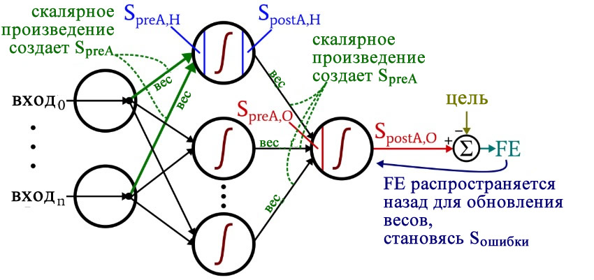
Вычисления, которые создают выходное значение, и в которых данные перемещаются слева направо на типовой схеме нейронной сети, составляют фрагмент «прямого распространения» работы системы. Вот код «прямого распространения»:
#####################
# обучение
#####################
for epoch in range(epoch_count):
    for sample in range(training_count):
        for node in range(H_dim):
            preActivation_H[node] = np.dot(training_data[sample,:], weights_ItoH[:, node])
            postActivation_H[node] = logistic(preActivation_H[node])

        preActivation_O = np.dot(postActivation_H, weights_HtoO)
        postActivation_O = logistic(preActivation_O)

        FE = postActivation_O - target_output[sample]
Первый цикл for позволяет нам проходить через несколько эпох. Внутри каждой эпохи, во втором цикле for, поочередно проходя по выборкам, мы вычисляем выходное значение для каждой выборки (то есть сигнал постактивации выходного узла). В третьем цикле for мы обращаемся индивидуально к каждому скрытому узлу, используя скалярное произведение для генерирования сигнала преактивации и функцию активации для генерирования сигнала постактивации.
После этого мы готовы вычислить сигнал преактивации для выходного узла (снова используя скалярное произведение), и мы применяем функцию активации для генерирования сигнала постактивации. Затем, чтобы вычислить итоговую ошибку, мы вычитаем целевое значение из значения полученного сигнала постактивации выходного узла.
Обратное распространение
После того, как мы выполнили расчеты для прямого распространения, настало время изменить направление. Во фрагменте программы с обратным распространением мы перемещаемся к весам от скрытых узлов к выходному узлу, а затем к весам от входного слоя к скрытому слою, перенося при этом информацию об ошибке для эффективного обучения сети.
        for H_node in range(H_dim):
            S_error = FE * logistic_deriv(preActivation_O)
            gradient_HtoO = S_error * postActivation_H[H_node]

            for I_node in range(I_dim):
                input_value = training_data[sample, I_node]
                gradient_ItoH = S_error * weights_HtoO[H_node] * logistic_deriv(preActivation_H[H_node]) * input_value

                weights_ItoH[I_node, H_node] -= LR * gradient_ItoH

            weights_HtoO[H_node] -= LR * gradient_HtoO
У нас есть два слоя для циклов for: один для весовых коэффициентов между скрытым и выходным слоями и один для весовых коэффициентов между входным и скрытым слоями. Сначала мы генерируем сигнал ошибки (Sошибки, S_error), который нам нужен для вычисления обоих градиентов, gradient_HtoO (от скрытого слоя к выходному) и gradient_ItoH (от входного слоя к скрытому), а затем мы обновляем весовые коэффициенты, вычитая градиент, умноженный на скорость обучения.
Обратите внимание, как веса между входным и скрытым слоями обновляются внутри цикла для значений между скрытым и выходным слоями. Мы начинаем с сигнала ошибки, который ведет обратно к одному из скрытых узлов, затем распространяем этот сигнал ошибки на все входные узлы, которые подключены к одному конкретному скрытому узлу:
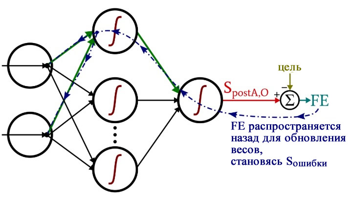
После того, как все весовые коэффициенты (как ItoH (от входного слоя к скрытому), так и HtoO (от скрытого слоя к выходному)), связанные с этим одним скрытым узлом, были обновлены, мы возвращаемся к началу и начинаем снова для следующего скрытого узла.
Также обратите внимание, что веса ItoH модифицируются перед весами HtoO. Мы используем текущий вес HtoO при расчете градиента, поэтому до выполнения расчетов мы не хотим изменять веса HtoO.
Заключение
Интересно задуматься о том, сколько теории ушло в эту относительно короткую программу на Python. Я надеюсь, что этот код на самом деле поможет вам понять, как мы можем программно реализовать нейронную сеть многослойный перцептрон.
Ниже приведен полный код программы.
import pandas
import numpy as np

def logistic(x):
    return 1.0/(1 + np.exp(-x))

def logistic_deriv(x):
    return logistic(x) * (1 - logistic(x))

LR = 1

I_dim = 3
H_dim = 4

epoch_count = 1

#np.random.seed(1)
weights_ItoH = np.random.uniform(-1, 1, (I_dim, H_dim))
weights_HtoO = np.random.uniform(-1, 1, H_dim)

preActivation_H = np.zeros(H_dim)
postActivation_H = np.zeros(H_dim)

training_data = pandas.read_excel('MLP_Tdata.xlsx')
target_output = training_data.output
training_data = training_data.drop(['output'], axis=1)
training_data = np.asarray(training_data)
training_count = len(training_data[:,0])

validation_data = pandas.read_excel('MLP_Vdata.xlsx')
validation_output = validation_data.output
validation_data = validation_data.drop(['output'], axis=1)
validation_data = np.asarray(validation_data)
validation_count = len(validation_data[:,0])

#####################
# обучение
#####################
for epoch in range(epoch_count):
    for sample in range(training_count):
        for node in range(H_dim):
            preActivation_H[node] = np.dot(training_data[sample,:], weights_ItoH[:, node])
            postActivation_H[node] = logistic(preActivation_H[node])

        preActivation_O = np.dot(postActivation_H, weights_HtoO)
        postActivation_O = logistic(preActivation_O)

        FE = postActivation_O - target_output[sample]

        for H_node in range(H_dim):
            S_error = FE * logistic_deriv(preActivation_O)
            gradient_HtoO = S_error * postActivation_H[H_node]

            for I_node in range(I_dim):
                input_value = training_data[sample, I_node]
                gradient_ItoH = S_error * weights_HtoO[H_node] * logistic_deriv(preActivation_H[H_node]) * input_value

                weights_ItoH[I_node, H_node] -= LR * gradient_ItoH

            weights_HtoO[H_node] -= LR * gradient_HtoO

#####################
# проверка
#####################
correct_classification_count = 0
for sample in range(validation_count):
    for node in range(H_dim):
        preActivation_H[node] = np.dot(validation_data[sample,:], weights_ItoH[:, node])
        postActivation_H[node] = logistic(preActivation_H[node])

    preActivation_O = np.dot(postActivation_H, weights_HtoO)
    postActivation_O = logistic(preActivation_O)

    if postActivation_O > 0.5:
        output = 1
    else:
        output = 0

    if output == validation_output[sample]:
        correct_classification_count += 1

print('Percentage of correct classifications:')
print(correct_classification_count*100/validation_count)
Теги
MLP, Multilayer Perceptron / Многослойный перцептронPythonМашинное обучение / Machine LearningНейросеть / Нейронная сетьОбработка прямого распространенияОбратное распространениеПерцептрон / PerceptronПрограммирование
В этой статье мы рассмотрим персептрон Розенблатта, надеюсь, вы получите интуитивное представление о том, как работает один персептрон в целях классификации. Это считается одним из крупнейших прорывов в истории искусственного интеллекта. Лично это была первая концепция машинного обучения, которую я узнал, которая пробудила мой интерес к этой области и дала мне основу для более легкого понимания других алгоритмов машинного обучения и искусственного интеллекта.
Если вы похожи на меня в том, что лучше понимаете логические концепции, прослеживая код, а не долго читая длинные уравнения с кучей обозначений, это чтение должно быть идеальным для вас. Если у вас нет опыта работы с Python, вы все равно можете изучить концепции высокого уровня. Но в любом случае, я сделаю все возможное, чтобы объяснить, что делает каждый отдельный фрагмент кода, чтобы, если у вас нет большого опыта работы с Python, вы могли следовать за ним.
ПРИМЕЧАНИЕ: если вы хотите загрузить полный код, используемый в этой статье, вы можете найти его здесь
Абстракция высокого уровня того, что делает персептрон
Мы сосредоточимся на использовании однослойного персептрона для классификации. этот метод машинного обучения считается «обучением с учителем», поскольку мы будем снабжать алгоритм помеченными обучающими данными. Это означает, что персептрону будет предоставлен набор данных, содержащий образцы с маркировкой «n» классов для обучения.
Чтобы дать вам лучшее представление, подумайте о том, как ребенок может научиться различать собаку и кошку. Допустим, мы представляем ему 100 различных изображений кошек и собак, рассказывая ему, что представляет собой каждое из них, и он сможет различать каждое из них на основе особенностей, которые он видит. Например, он заключает, что у кошек короткие уши, а у собак длинные. Теперь, конечно, человеческий разум не смотрит на кошку и не говорит: «Если уши имеют длину от 2,345 до 3,67 см, это кошка», но именно так это может увидеть персептрон.
Если вы открывали любую другую статью или видео о персептронах до того, как попали сюда, скорее всего, вы видели эту диаграмму. Давайте сначала рассмотрим каждый компонент здесь, а затем рассмотрим сам процесс.
x и w: каждый X, представленный нижним индексом «i», здесь представляет функцию, поэтому здесь у нас есть «m» количество функций, опять же в сценарии «кошка-собака» это может быть длина уха. Каждая функция связана с весом, с математической точки зрения, вес каждой функции — это ее коэффициент. «Вес», как следует из названия, можно рассматривать как представление уровня влияния, которое оказывает эта функция. «Обучающая часть» любого алгоритма машинного обучения — это процесс нахождения оптимального значения каждого веса.
Чистый вход: чистый вход (обозначенный сигмой на диаграмме) представляет собой скалярную сумму признаков и весов:

Функция активации: это последний шаг в нашей модели классификации, функция сетевого ввода, на основе которой мы можем «классифицировать» данные с помощью двоичного вывода. Сама функция может иметь разные формы, но для простоты мы сосредоточимся на «шаговой функции», которая является самой простой реализацией; как следует из формы на диаграмме и названия, модель будет делать прогноз классификации на основе того, пересекает ли чистая входная информация определенное пороговое значение.
Ошибка: в процессе обучения модель делает прогноз, используя определенные нами компоненты, и проверяет правильность вывода. На основании ошибки мы обновляем наши веса. в конечном итоге наша цель состоит в том, чтобы свести к минимуму ошибки с каждой итерацией обучения, чтобы наша модель сходилась.
Собираем все вместе
Теперь давайте разберемся с этой моделью. Итак, мы хотим научить персептрон классифицировать два отдельных объекта с учетом ряда признаков. Алгоритм выполняет определенное количество итераций, выполняя шаги, описанные на диаграмме, обновляя веса на основе ошибки, полученной на каждой итерации.
После завершения процесса обучения у нас есть оптимизированный набор весов, который можно использовать вместе с функциями для классификации неразмеченных данных. Пока что это все очень абстрактные концепции, если вы новичок в нейронных сетях, я не ожидаю, что вы сможете смоделировать алгоритм классификатора персептрона, но важно иметь краткий обзор этих концепций, прежде чем погрузиться в алгоритмическая реализация.
Реализация бинарного классификатора персептрона в Python
Изучив концепции высокого уровня, мы можем теперь изучить детали очень простой реализации персептрона в python, чтобы закрепить наше понимание.
Прежде всего, давайте быстро пробежимся по библиотекам, которые мы будем использовать:
- Numpy: это одна из наиболее распространенных библиотек, используемых в приложениях для работы с данными. Она позволяет нам создавать «массивы numpy», похожие на списки, но их реализация позволяет нам выполнять вычисления с этими массивами.
- Случайно: мы будем использовать случайный выбор для инициализации наших весов.
- Pandas: pandas также является очень мощной библиотекой для работы с данными, но в нашем случае мы будем использовать pandas просто для импорта нашего примера набора данных.
- Matplotlib: наконец, мы будем использовать matplotlib для визуализации концепций.
Пример набора данных:
В этом примере мы будем использовать набор данных «цветок ириса». Эти данные содержат 3 разных цветка с 50 различными образцами для каждого типа цветка, содержащими 4 признака, которые численно описывают цветок (например, длину лепестка). Давайте импортируем и просмотрим этот набор данных, чтобы лучше понять, с чем мы имеем дело.
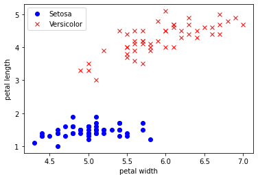
Для простоты мы будем использовать 2 из 3 цветов, поэтому наш персептрон, по сути, будет предсказывать, является ли цветок Setosa или Versicolor, основываясь на двух характеристиках (то есть ширине и длине лепестков). На графике легко заметить, что наши данные могут быть разделены линейной линией, и это то, что наша модель попытается изучить. Обратите внимание: поскольку мы сохраняем базовую модель, которую мы собираемся использовать, она сможет классифицировать только линейно разделяемые данные.
Импортировав образцы данных и библиотеки, мы можем приступить к работе с нашей моделью:
здесь мы определяем новый класс «персептрон», инициализируя скорость обучения (eta) и количество итераций (n_iter). Эти два значения называются гиперпараметрами, скорость обучения — это число с плавающей запятой от 0 до 1, а количество итераций — целое число. Оптимальное значение этих двух переменных зависит от самой проблемы. Оптимизация гиперпараметров — это тема для отдельной статьи, а пока все, что нам нужно знать об этих двух, это следующее:
- Скорость обучения (эта): интуиция здесь такова, что если скорость обучения слишком высока, наша модель выйдет за рамки допустимого.
- Количество итераций (n_iter): это количество итераций, которые наш алгоритм будет выполнять с обучающими данными.
Теперь давайте возьмем блок-схему, которую мы обсуждали ранее, и переведем ее в код Python:
В нашей модели перцептрона определены три функции. Функция fit() — это в основном место, где происходит все обучение, и веса обновляются итеративно, так что после завершения обучения у нас должен быть массив размера 3, содержащий веса для функций, и последнее значение «смещение», которое эквивалентно «у-перехвату».
Функция подгонки состоит из двух вложенных циклов. Внешний цикл — это то, сколько раз алгоритм будет работать с нашим тренировочным набором, а внутренний цикл — это фактический «обход тренировочного набора». Здесь параметр «X» представляет собой двумерный массив numpy, содержащий значения функций, а «y» — это метка для каждой строки функций. Мы используем встроенное ключевое слово python zip(X, y), чтобы в основном просмотреть каждый помеченный образец.
Наиболее неотъемлемым компонентом нашего процесса обучения является обновление веса. Обновление определяется как:

Это можно рассматривать как математическое представление того, насколько правильным или неправильным было предсказание нашей модели. Чтобы лучше понять это, мы можем рассмотреть четыре возможных результата этого уравнения. Как мы упоминали ранее, каждый цветок выражается числовым значением либо 1, либо -1, где -1 — это «сетоза», а 1 — «разноцветный».
теперь в нашем внутреннем цикле компилятор просматривает ряд образцов и пытается «предсказать», что этот образец использует с заданными функциями и текущими весами нашей модели.
Возьмем два сценария, в которых наша модель неверна (мы игнорируем eta, поскольку это просто константа):
- (1)-(-1) = 2
- (-1)-(1) = -2
Что касается того, когда наша модель правильная, мы получаем, другими словами, и метка, и прогноз имеют одинаковое значение:
- (1)-(1) = 0
- (-1)-(-1) = 0
Когда прогноз неверен, веса обновляются в направлении ошибки. Тогда как, если это правильно, результат равен нулю, а веса остаются неизменными.
Обучение нашего персептрона
надеюсь, теперь у вас есть представление о том, что делает модель, вы также можете обратиться к комментариям в коде, если что-то неясно. Итак, приступим к обучению:
сначала мы инициализируем наш персептрон как новый объект. Мы уже импортировали наш набор данных, но здесь мы определяем его в формате, который может быть понят нашей функцией fit() (принимая функции в столбцах с индексами 0 и 2 как двумерный массив numpy и 4-й index, который является классом образца в отдельном массиве numpy). Мы также используем функцию np.where, чтобы изменить строковые значения класса на 1 (лишай) и -1 (сетоза). Затем мы можем запустить функцию fit() для наших значений X и y, чтобы обучить наш персептрон, наконец, после определенного количества итераций у нас должен быть пустой массив, содержащий наш оптимальный вес, и теперь мы можем вызывать predict() на немаркированном образце, и наш персептрон классифицирует его.
Ошибки построения
Определенная переменная self.errors_ на самом деле не способствует нашему процессу обучения, но мы можем использовать ее для построения графика количества ошибок на каждой итерации:
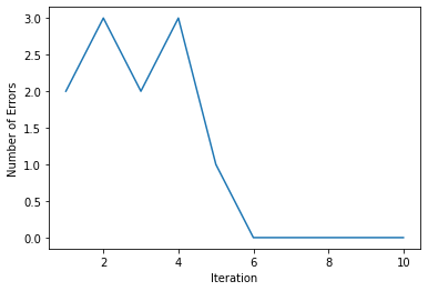
Из графика видно, что наша модель сошлась после 6-й итерации. Это может немного меняться с каждым запуском, так как мы рандомизируем наши начальные веса.
Резюме и выводы
В этой статье мы рассмотрели абстрактные концепции очень простого персептрона, а затем подробно рассмотрели его реализацию на Python. Как я уже упоминал во введении, эта статья в основном предназначена для всех, кто знаком с python и хочет заняться машинным обучением. Исходя из моего личного опыта, я считаю, что лучше всего реализовать алгоритм с нуля, если я хочу глубже понять концепцию. Так что не стесняйтесь экспериментировать с кодом, изменяя гиперпараметры с помощью print() и графиков, чтобы лучше понять каждый компонент.
В следующей части этой статьи я подробнее остановлюсь на аспектах визуализации. Анимация процесса обучения в виде графиков, чтобы лучше понять контролируемое обучение. Имейте в виду, что это очень простая форма контролируемого машинного обучения, и, конечно же, наша модель имеет много ограничений. В будущем мы рассмотрим более сложные модели, расширяющие модель, описанную здесь.
Надеюсь, вы нашли это познавательным!
использованная литература
2015. Глава 2. Обучение простым алгоритмам машинного обучения для классификации. В С. Рашка, Машинное обучение Python (стр. 63–83). Издательство Пакет.
| title | date | categories | tags | |||
|---|---|---|---|---|---|---|
|
Linking maths and intuition: Rosenblatt’s Perceptron in Python |
2019-07-23 |
svms |
|
According to Wikipedia, Frank Rosenblatt is an «American psychologist notable in the field of artificial intelligence».
And notable, he is.
Rosenblatt is the inventor of the so-called Rosenblatt Perceptron, which is one of the first algorithms for supervised learning, invented in 1958 at the Cornell Aeronautical Laboratory.
The blogs I write on MachineCurve.com are educational in two ways. First, I use them to structure my thoughts on certain ML related topics. Second, if they help me, they could help others too. This blog is one of the best examples: it emerged from my struggle to identify why it is difficult to implement Rosenblatt’s Perceptron with modern machine learning frameworks.
Turns out that has to do with the means of optimizing one’s model — a.k.a. the Perceptron Learning Rule vs Stochastic Gradient Descent. I’m planning to dive into this question in detail in another blog. This article describes the work I preformed before being able to answer it — or, programming a Perceptron myself, understanding how it attempts to find the best decision boundary. It provides a tutorial for implementing the Rosenblatt Perceptron yourself.
I will first introduce the Perceptron in detail by discussing some of its history as well as its mathematical foundations. Subsequently, I will move on to the Perceptron Learning Rule, demonstrating how it improves over time. This is followed by a Python based Perceptron implementation that is finally demonstrated with a real dataset.
Of course, if you want to start working with the Perceptron right away, you can find example code for the Rosenblatt Perceptron in the first section.
If you run into questions during the read, or if you have any comments, please feel free to write a comment in the comment box near the bottom 👇 I’m happy to provide my thoughts and improve this post whenever I’m wrong. I hope to hear from you!
Update 13/Jan/2021: Made article up-to-date. Added quick example to answer question how to implement Rosenblatt Perceptron with Python? Performed changes to article structure. Added links to other articles. It’s now ready for 2021!
[toc]
Answer: implementing Rosenblatt Perceptron with Python
Some people just want to start with code before they read further. That’s why in this section, you’ll find a fully functional example of the Rosenblatt Perceptron, created with Python. It shows a class that is initialized, that has a training loop (train definition) and which can generate predictions once trained (through predict). If you want to understand the Perceptron in more detail, make sure to read the rest of this tutorial too!
import numpy as np

# Basic Rosenblatt Perceptron implementation
class RBPerceptron:

  # Constructor
  def __init__(self, number_of_epochs = 100, learning_rate = 0.1):
    self.number_of_epochs = number_of_epochs
    self.learning_rate = learning_rate

  # Train perceptron
  def train(self, X, D):
    # Initialize weights vector with zeroes
    num_features = X.shape[1]
    self.w = np.zeros(num_features + 1)
    # Perform the epochs
    for i in range(self.number_of_epochs):
      # For every combination of (X_i, D_i)
      for sample, desired_outcome in zip(X, D):
        # Generate prediction and compare with desired outcome
        prediction    = self.predict(sample)
        difference    = (desired_outcome - prediction)
        # Compute weight update via Perceptron Learning Rule
        weight_update = self.learning_rate * difference
        self.w[1:]    += weight_update * sample
        self.w[0]     += weight_update
    return self

  # Generate prediction
  def predict(self, sample):
    outcome = np.dot(sample, self.w[1:]) + self.w[0]
    return np.where(outcome > 0, 1, 0)
A small introduction — what is a Perceptron?
A Perceptron is a binary classifier that was invented by Frank Rosenblatt in 1958, working on a research project for Cornell Aeronautical Laboratory that was US government funded. It was based on the recent advances with respect to mimicing the human brain, in particular the MCP architecture that was recently invented by McCulloch and Pitts.
This architecture attempted to mimic the way neurons operate in the brain: given certain inputs, they fire, and their firing behavior can change over time. By allowing the same to happen in an artificial neuron, researchers at the time argued, machines could become capable of approximating human intelligence.
…well, that was a slight overestimation, I’d say 😄 Nevertheless, the Perceptron lies at the basis of where we’ve come today. It’s therefore a very interesting topic to study deeper. Next, I will therefore scrutinize its mathematical building blocks, before moving on to implementing one in Python.
[ad]
Mathematical building blocks
When you train a supervised machine learning model, it must somehow capture the information that you’re giving it. The Perceptron does this by means of a weights vector, or **w** that determines the exact position of the decision boundary and is learnt from the data.
If you input new data, say in an input vector **x**, you’ll simply have to pinpoint this vector with respect to the learnt weights, to decide on the class.
Mathematically, this is represented as follows:
[mathjax]
begin{equation} f(x) = begin{cases} 1, & text{if} textbf{w}cdottextbf{x}+b > 0 \ 0, & text{otherwise} \ end{cases} end{equation}
Here, you can see why it is a binary classifier: it simply determines the data to be part of class ‘0’ or class ‘1’. This is done based on the output of the multiplication of the weights and input vectors, with a bias value added.
When you multiply two vectors, you’re computing what is called a dot product. A dot product is the sum of the multiplications of the individual scalars in the vectors, pair-wise. This means that e.g. [latex]w_1x_1[/latex] is computed and summated together with [latex]w_2x_2[/latex], [latex]w_3x_3[/latex] and so on … until [latex]w_nx_n[/latex]. Mathematically:
begin{equation} begin{split} &z=sum_{i=1}^{n} w_nx_n + b \ &= w_1x_1 + … + w_nx_n + b \ end{split} end{equation}
When this output value is larger than 0, it’s class 1, otherwise it’s class 0. In other words: binary classification.
The Perceptron, visually
Visually, this looks as follows:

All right — we now have a mathematical structure for automatically deciding about the class. Weights vector **w** and bias value _b_ are used for setting the decision boundary. We did however not yet cover how the Perceptron is updated. Let’s find out now!
Before optimizing: moving the bias into the weights vector
Rosenblatt did not only provide the model of the perceptron, but also the method for optimizing it.
This however requires that we first move the bias value into the weights vector.
This sounds strange, but it is actually a very elegant way of making the equation simpler.
[ad]
As you recall, this is how the Perceptron can be defined mathematically:
begin{equation} f(x) = begin{cases} 1, & text{if} textbf{w}cdottextbf{x}+b > 0 \ 0, & text{otherwise} \ end{cases} end{equation}
Of which [latex]textbf{w}cdottextbf{x}+b[/latex] could be written as:
begin{equation} begin{split} &z=sum_{i=1}^{n} w_nx_n + b \ &= w_1x_1 + … + w_nx_n + b \ end{split} end{equation}
We now add the bias to the weights vector as [latex]w_0[/latex] and choose [latex]x_0 = 1[/latex]. This looks as follows:

This allows us to rewrite [latex]z[/latex] as follows — especially recall that [latex]w_0 = b[/latex] and [latex]x_0 = 1[/latex]:
begin{equation} begin{split} & z = sum_{i=0}^{n} w_nx_n \ & = w_0x_0 + w_1x_1 + … + w_nx_n \ & = w_0x_0 + w_1x_1 + … + w_nx_n \ & = 1b + w_1x_1 + … + w_nx_n \ & = w_1x_1 + … + w_nx_n + b end{split} end{equation}
As you can see, it is still equal to the original way of writing it:
begin{equation} begin{split} &z=sum_{i=1}^{n} w_nx_n + b \ &= w_1x_1 + … + w_nx_n + b \ end{split} end{equation}
This way, we got rid of the bias [latex]b[/latex] in our main equation, which will greatly help us with what we’ll do now: update the weights in order to optimize the model.
Training the model
We’ll use what is called the Perceptron Learning Rule for that purpose. But first, we need to show you how the model is actually trained — by showing the pseudocode for the entire training process.
We’ll have to make a couple assumptions at first:
- There is the weights vector
wwhich, at the beginning, is uninitialized. - You have a set of training values, such as [latex]T = { (x_1, d_1), (x_2, d_2), …, (x_n, d_n) }[/latex]. Here, [latex]x_n[/latex] is a specific feature vector, while [latex]d_n[/latex] is the corresponding target value.
- We ensure that [latex]w_0 = b[/latex] and [latex]x_0 = 1[/latex].
- We will have to configure a learning rate or [latex]r[/latex], or by how much the model weights improve. This is a number between 0 and 1. We use [latex]r = 0.1[/latex] in the Python code that follows next.
This is the pseudocode:
- Initialize the weights vector
**w**to zeroes or random numbers. - For every [latex](x_n, d_n)[/latex] in [latex]D[/latex]:
- Compute the output value for the input vector [latex]x_n[/latex]. Mathematically, that’s [latex]d’_n: f(x_n) = w_nx_n[/latex].
- Compare the output value [latex]d’_n[/latex] with target value [latex]d_n[/latex].
- Update the weights according to the Perceptron Learning Rule: [latex]w_text{n,i}(t+1) = w_text{n,i}(t) + r cdot (d_n — d’_n) cdot x_text{n,i}[/latex] for all features (scalars) [latex]0 leq i leq|w_n|[/latex].
Or, in plain English:
- First initialize the weights randomly or to zeroes.
- Iterate over every feature in the data set.
- Compute the output value.
- Compare if it matches, and ‘push’ the weights into the right direction (i.e. the [latex]d_n — d’_n[/latex] part) slightly with respect to [latex]x_text{n,i}[/latex], as much as the learning rate [latex]r[/latex] allows.
This means that the weights are updated for every sample from the dataset.
This process may be repeated until some criterion is reached, such as a specific number of errors, or — if you are adventurous — full convergence (i.e., the number of errors is 0).
Perceptron in Python
Now let’s see if we can code a Perceptron in Python. Create a new folder and add a file named p.py. In it, let’s first import numpy, which we’ll need for some number crunching:
We’ll create a class that is named RBPerceptron, or Rosenblatt’s Perceptron. Classes in Python have a specific structure: they must be defined as such (by using class) and can contain Python definitions which must be coupled to the class through self. Additionally, it may have a constructor definition, which in Python is called __init__.
Class definition and constructor
So let’s code the class:
# Basic Rosenblatt Perceptron implementation
class RBPerceptron:
Next, we want to allow the engineer using our Perceptron to configure it before he or she starts the training process. We would like them to be able to configure two variables:
- The number of epochs, or rounds, before the model stops the training process.
- The learning rate [latex]r[/latex], i.e. the determinant for the size of the weight updates.
We’ll do that as follows:
  # Constructor
  def __init__(self, number_of_epochs = 100, learning_rate = 0.1):
    self.number_of_epochs = number_of_epochs
    self.learning_rate = learning_rate
The __init__ definition nicely has a self reference, but also two attributes: number_of_epochs and learning_rate. These are preconfigured, which means that if those values are not supplied, those values serve as default ones. By default, the model therefore trains for 100 epochs and has a default learning rate of 0.1
However, since the user can manually provide those, they must also be set. We need to use them globally: the number of epochs and the learning rate are important for the training process. By consequence, we cannot simply keep them in the context of our Python definition. Rather, we must add them to the instance variables of the class. This can be done by assigning them to the class through self.
[ad]
The training definition
All right, the next part — the training definition:
  # Train perceptron
  def train(self, X, D):
    # Initialize weights vector with zeroes
    num_features = X.shape[1]
    self.w = np.zeros(num_features + 1)
    # Perform the epochs
    for i in range(self.number_of_epochs):
      # For every combination of (X_i, D_i)
      for sample, desired_outcome in zip(X, D):
        # Generate prediction and compare with desired outcome
        prediction    = self.predict(sample)
        difference    = (desired_outcome - prediction)
        # Compute weight update via Perceptron Learning Rule
        weight_update = self.learning_rate * difference
        self.w[1:]    += weight_update * sample
        self.w[0]     += weight_update
    return self
The definition it self must once again have a self reference, which is provided. However, it also requires the engineer to pass two attributes: X, or the set of input samples [latex]x_1 … x_n[/latex], as well as D, which are their corresponding targets.
Within the definition, we first initialize the weights vector as discussed above. That is, we assign it with zeroes, and it is num_features + 1 long. This way, it can both capture the features [latex]x_1 … x_n[/latex] as well as the bias [latex]b[/latex] which was assigned to [latex]x_0[/latex].
Next, the training process. This starts by creating a for statement that simply ensures that the program iterates over the number_of_epochs that were configured by the user.
During one iteration, or epoch, every combination of [latex](x_i, d_i)[/latex] is iterated over. In line with the pseudocode algorithm, a prediction is generated, the difference is computed, and the weights are updated accordingly.
After the training process has finished, the model itself is returned. This is not necessary, but is relatively convenient for later use by the ML engineer.
Generating predictions
Finally, the model must also be capable of generating predictions, i.e. computing the dot product [latex]textbf{w}cdottextbf{x}[/latex] (where [latex]b[/latex] is included as [latex]w_0[/latex]).
We do this relatively elegantly, thanks to another example of the Perceptron algorithm provided by Sebastian Raschka: we first compute the dot product for all weights except [latex]w_0[/latex] and subsequently add this one as the bias weight. Most elegantly, however, is how the prediction is generated: with np.where. This allows an engineer to generate predictions for a batch of samples [latex]x_i[/latex] at once. It looks as follows:
  # Generate prediction
  def predict(self, sample):
    outcome = np.dot(sample, self.w[1:]) + self.w[0]
    return np.where(outcome > 0, 1, 0)
Final code
All right — when integrated, this is our final code.
You can also check it out on GitHub.
import numpy as np

# Basic Rosenblatt Perceptron implementation
class RBPerceptron:

  # Constructor
  def __init__(self, number_of_epochs = 100, learning_rate = 0.1):
    self.number_of_epochs = number_of_epochs
    self.learning_rate = learning_rate

  # Train perceptron
  def train(self, X, D):
    # Initialize weights vector with zeroes
    num_features = X.shape[1]
    self.w = np.zeros(num_features + 1)
    # Perform the epochs
    for i in range(self.number_of_epochs):
      # For every combination of (X_i, D_i)
      for sample, desired_outcome in zip(X, D):
        # Generate prediction and compare with desired outcome
        prediction    = self.predict(sample)
        difference    = (desired_outcome - prediction)
        # Compute weight update via Perceptron Learning Rule
        weight_update = self.learning_rate * difference
        self.w[1:]    += weight_update * sample
        self.w[0]     += weight_update
    return self

  # Generate prediction
  def predict(self, sample):
    outcome = np.dot(sample, self.w[1:]) + self.w[0]
    return np.where(outcome > 0, 1, 0)
Testing with a dataset
All right, let’s now test our implementation of the Perceptron. For that, we’ll need a dataset first. Let’s generate one with Python. Go to the same folder as p.py and create a new one, e.g. dataset.py. Use this file for the next steps.
Generating the dataset
We’ll first import numpy and generate 50 zeros and 50 ones.
We then combine them into the targets list, which is now 100 long.
We’ll then use the normal distribution to generate two samples that do not overlap of both 50 samples.
Finally, we concatenate the samples into the list of input vectors X and set the desired targets D to the targets generated before.
# Import libraries
import numpy as np

# Generate target classes {0, 1}
zeros = np.zeros(50)
ones = zeros + 1
targets = np.concatenate((zeros, ones))

# Generate data
small = np.random.normal(5, 0.25, (50,2))
large = np.random.normal(6.5, 0.25, (50,2))

# Prepare input data
X = np.concatenate((small,large))
D = targets
Visualizing the dataset
It’s always nice to get a feeling for the data you’re working with, so let’s first visualize the dataset:
import matplotlib.pyplot as plt
plt.scatter(small[:,0], small[:,1], color='blue')
plt.scatter(large[:,0], large[:,1], color='red')
plt.show()
It should look like this:

Let’s next train our Perceptron with the entire training set X and the corresponding desired targets D.
[ad]
We must first initialize our Perceptron for this purpose:
from p import RBPerceptron
rbp = RBPerceptron(600, 0.1)
Note that we use 600 epochs and set a learning rate of 0.1. Let’s now train our model:
trained_model = rbp.train(X, D)
The training process should be completed relatively quickly. We can now visualize the Perceptron and its decision boundary with a library called mlxtend — once again the credits for using this library go out to Sebastian Raschka.
If you don’t have it already, install it first by means of pip install mlxtend.
Subsequently, add this code:
from mlxtend.plotting import plot_decision_regions
plot_decision_regions(X, D.astype(np.integer), clf=trained_model)
plt.title('Perceptron')
plt.xlabel('X1')
plt.ylabel('X2')
plt.show()
You should now see the same data with the Perceptron decision boundary successfully separating the two classes:

There you go, Rosenblatt’s Perceptron in Python!
References
Bernard (2018, December). Align equation left. Retrieved from https://tex.stackexchange.com/questions/145657/align-equation-left
Raschka, S. (2015, March 24). Single-Layer Neural Networks and Gradient Descent. Retrieved from https://sebastianraschka.com/Articles/2015_singlelayer_neurons.html#artificial-neurons-and-the-mcculloch-pitts-model
Perceptron. (2003, January 22). Retrieved from https://en.wikipedia.org/wiki/Perceptron#Learning_algorithm
First introduced by Rosenblatt in 1958, The Perceptron: A Probabilistic Model for Information Storage and Organization in the Brain is arguably the oldest and most simple of the ANN algorithms. Following this publication, Perceptron-based techniques were all the rage in the neural network community. This paper alone is hugely responsible for the popularity and utility of neural networks today.
But then, in 1969, an “AI Winter” descended on the machine learning community that almost froze out neural networks for good. Minsky and Papert published Perceptrons: an introduction to computational geometry, a book that effectively stagnated research in neural networks for almost a decade — there is much controversy regarding the book (Olazaran, 1996), but the authors did successfully demonstrate that a single layer Perceptron is unable to separate nonlinear data points.
Given that most real-world datasets are naturally nonlinearly separable, this it seemed that the Perceptron, along with the rest of neural network research, might reach an untimely end.
Between the Minsky and Papert publication and the broken promises of neural networks revolutionizing industry, the interest in neural networks dwindled substantially. It wasn’t until we started exploring deeper networks (sometimes called multi-layer perceptrons) along with the backpropagation algorithm (Werbos and Rumelhart et al.) that the “AI Winter” in the 1970s ended and neural network research started to heat up again.
All that said, the Perceptron is still a very important algorithm to understand as it sets the stage for more advanced multi-layer networks. We’ll start this section with a review of the Perceptron architecture and explain the training procedure (called the delta rule) used to train the Perceptron. We’ll also look at the termination criteria of the network (i.e., when the Perceptron should stop training). Finally, we’ll implement the Perceptron algorithm in pure Python and use it to study and examine how the network is unable to learn nonlinearly separable datasets.
![]()
Looking for the source code to this post?
Jump Right To The Downloads Section
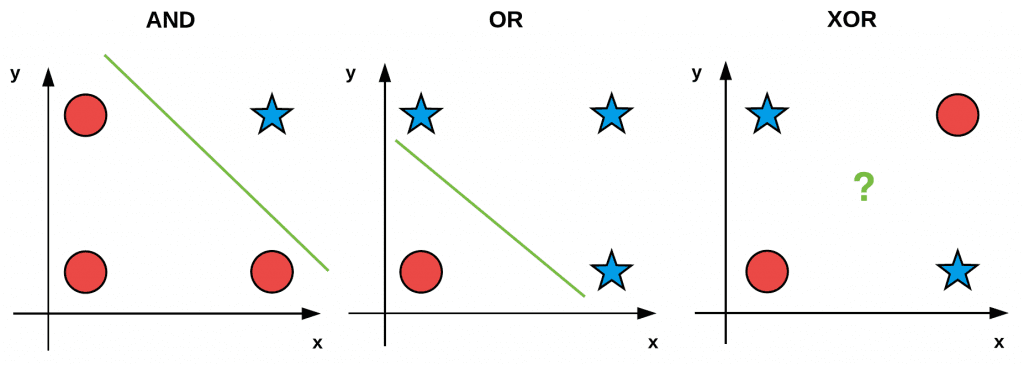
AND, OR, and XOR Datasets
Before we study the Perceptron itself, let’s first discuss “bitwise operations,” including AND, OR, and XOR (exclusive OR). If you’ve taken an introductory level computer science course before you might already be familiar with bitwise functions.
Bitwise operators and associated bitwise datasets accept two input bits and produce a final output bit after applying the operation. Given two input bits, each potentially taking on a value of 0 or 1, there are four possible combinations of these two bits — Table 1 provides the possible input and output values for AND, OR, and XOR:
| x0 | x1 | x0&x1 | x0 | x1 | x0|x1 | x0 | x1 | x0∧x1 |
|---|---|---|---|---|---|---|---|---|
| 0 | 0 | 0 | 0 | 0 | 0 | 0 | 0 | 0 |
| 0 | 1 | 0 | 0 | 1 | 1 | 0 | 1 | 1 |
| 1 | 0 | 0 | 1 | 0 | 1 | 1 | 0 | 1 |
| 1 | 1 | 1 | 1 | 1 | 1 | 1 | 1 | 0 |
As we can see on the left, a logical AND is true if and only if both input values are 1. If either of the input values is 0, the AND returns 0. Thus, there is only one combination, x0 = 1 and x1 = 1 when the output of AND is true.
In the middle, we have the OR operation which is true when at least one of the input values is 1. Thus, there are three possible combinations of the two bits x0 and x1 that produce a value of y = 1.
Finally, the right displays the XOR operation which is true if and only if one if the inputs is 1 but not both. While OR had three possible situations where y = 1, XOR only has two.
We often use these simple “bitwise datasets” to test and debug machine learning algorithms. If we plot and visualize the AND, OR, and XOR values (with red circles being zero outputs and blue stars one outputs) in Figure 1, you’ll notice an interesting pattern:
Both AND and OR are linearly separable — we can clearly draw a line that separates the 0 and 1 classes — the same is not true for XOR. Take the time now to convince yourself that it is not possible to draw a line that cleanly separates the two classes in the XOR problem. XOR is, therefore, an example of a nonlinearly separable dataset.
Ideally, we would like our machine learning algorithms to be able to separate nonlinear classes as most datasets encountered in the real world are nonlinear. Therefore, when constructing, debugging, and evaluating a given machine learning algorithm, we may use the bitwise values x0 and x1 as our design matrix and then try to predict the corresponding y values.
Unlike our standard procedure of splitting our data into training and testing splits, when using bitwise datasets we simply train and evaluate our network on the same set of data. Our goal here is simply to determine if it’s even possible for our learning algorithm to learn the patterns in the data. As we’ll find out, the Perceptron algorithm can correctly classify the AND and OR functions but fails to classify the XOR data.
Perceptron Architecture
Rosenblatt (1958) defined a Perceptron as a system that learns using labeled examples (i.e., supervised learning) of feature vectors (or raw pixel intensities), mapping these inputs to their corresponding output class labels.
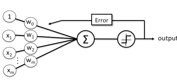
In its simplest form, a Perceptron contains N input nodes, one for each entry in the input row of the design matrix, followed by only one layer in the network with just a single node in that layer (Figure 2).
There exist connections and their corresponding weights w1, w2, …, wi from the input xi’s to the single output node in the network. This node takes the weighted sum of inputs and applies a step function to determine the output class label. The Perceptron outputs either a 0 or a 1 — 0 for class #1 and 1 for class #2; thus, in its original form, the Perceptron is simply a binary, two-class classifier.

1. Initialize our weight vector w with small random values
2. Until Perceptron converges:
(a) Loop over each feature vector xj and true class label di in our training set D
(b) Take x and pass it through the network, calculating the output value: yj = f(w(t) · xj)
(c) Update the weights w: wi(t +1) = wi(t) +α(dj −yj)xj,i for all features 0 <= i <= n
Perceptron Training Procedure and the Delta Rule
Training a Perceptron is a fairly straightforward operation. Our goal is to obtain a set of weights w that accurately classifies each instance in our training set. In order to train our Perceptron, we iteratively feed the network with our training data multiple times. Each time the network has seen the full set of training data, we say an epoch has passed. It normally takes many epochs until a weight vector w can be learned to linearly separate our two classes of data.
The pseudocode for the Perceptron training algorithm can be found below:
The actual “learning” takes place in Steps 2b and 2c. First, we pass the feature vector xj through the network, take the dot product with the weights w and obtain the output yj. This value is then passed through the step function which will return 1 if x > 0 and 0 otherwise.
Now we need to update our weight vector w to step in the direction that is “closer” to the correct classification. This update of the weight vector is handled by the delta rule in Step 2c.
The expression (dj −yj) determines if the output classification is correct or not. If the classification is correct, then this difference will be zero. Otherwise, the difference will be either positive or negative, giving us the direction in which our weights will be updated (ultimately bringing us closer to the correct classification). We then multiply (dj − yj) by xj, moving us closer to the correct classification.
The value α is our learning rate and controls how large (or small) of a step we take. It’s critical that this value is set correctly. A larger value of α will cause us to take a step in the right direction; however, this step could be too large, and we could easily overstep a local/global optimum.
Conversely, a small value of α allows us to take tiny baby steps in the right direction, ensuring we don’t overstep a local/global minimum; however, these tiny baby steps may take an intractable amount of time for our learning to converge.
Finally, we add in the previous weight vector at time t, wj(t) which completes the process of “stepping” towards the correct classification. If you find this training procedure a bit confusing, don’t worry.
Perceptron Training Termination
The Perceptron training process is allowed to proceed until all training samples are classified correctly or a preset number of epochs is reached. Termination is ensured if α is sufficiently small and the training data is linearly separable.
So, what happens if our data is not linearly separable or we make a poor choice in α? Will training continue infinitely? In this case, no — we normally stop after a set number of epochs has been hit or if the number of misclassifications has not changed in a large number of epochs (indicating that the data is not linearly separable). For more details on the perceptron algorithm, please refer to either Andrew Ng’s Stanford lecture or the introductory chapters of Mehrota et al. (1997).
Implementing the Perceptron in Python
Now that we have studied the Perceptron algorithm, let’s implement the actual algorithm in Python. Create a file named perceptron.py in your pyimagesearch.nn package — this file will store our actual Perceptron implementation:
|--- pyimagesearch
|    |--- __init__.py
|    |--- nn
|    |    |--- __init__.py
|    |    |--- perceptron.py
After you’ve created the file, open it, and insert the following code:
# import the necessary packages
import numpy as np

class Perceptron:
	def __init__(self, N, alpha=0.1):
		# initialize the weight matrix and store the learning rate
		self.W = np.random.randn(N + 1) / np.sqrt(N)
		self.alpha = alpha
Line 5 defines the constructor to our Perceptron class, which accepts a single required parameter followed by a second optional one:
N: The number of columns in our input feature vectors. In the context of our bitwise datasets, we’ll setNequal to two since there are two inputs.alpha: Our learning rate for the Perceptron algorithm. We’ll set this value to0.1by default. Common choices of learning rates are normally in the range α = 0.1, 0.01, 0.001.
Line 7 files our weight matrix W with random values sampled from a “normal” (Gaussian) distribution with zero mean and unit variance. The weight matrix will have N +1 entries, one for each of the N inputs in the feature vector, plus one for the bias. We divide W by the square-root of the number of inputs, a common technique used to scale our weight matrix, leading to faster convergence. We will cover weight initialization techniques later in this chapter.
Next, let’s define the step function:
	def step(self, x):
		# apply the step function
		return 1 if x > 0 else 0
This function mimics the behavior of the step equation — if x is positive we return 1, otherwise, we return 0.
To actually train the Perceptron we’ll define a function named fit. If you have any previous experience with machine learning, Python, and the scikit-learn library then you’ll know that it’s common to name your training procedure function fit, as in “fit a model to the data”:
	def fit(self, X, y, epochs=10):
		# insert a column of 1's as the last entry in the feature
		# matrix -- this little trick allows us to treat the bias
		# as a trainable parameter within the weight matrix
		X = np.c_[X, np.ones((X.shape[0]))]
The fit method requires two parameters followed by a single optional one:
The X value is our actual training data. The y variable is our target output class labels (i.e., what our network should be predicting). Finally, we supply epochs, the number of epochs our Perceptron will train for.
Line 18 applies the bias trick by inserting a column of ones into the training data, which allows us to treat the bias as a trainable parameter directly inside the weight matrix.
Next, let’s review the actual training procedure:
		# loop over the desired number of epochs
		for epoch in np.arange(0, epochs):
			# loop over each individual data point
			for (x, target) in zip(X, y):
				# take the dot product between the input features
				# and the weight matrix, then pass this value
				# through the step function to obtain the prediction
				p = self.step(np.dot(x, self.W))

				# only perform a weight update if our prediction
				# does not match the target
				if p != target:
					# determine the error
					error = p - target

					# update the weight matrix
					self.W += -self.alpha * error * x
On Line 21, we start looping over the desired number of epochs. For each epoch, we also loop over each individual data point x and output target class label (Line 23).
Line 27 takes the dot product between the input features x and the weight matrix W, then passes the output through the step function to obtain the prediction by the Perceptron.
Applying the same training procedure detailed in Figure 3, we only perform a weight update if our prediction does not match the target (Line 31). If this is the case, we determine the error (Line 33) by computing the sign (either positive or negative) via the difference operation.
Updating the weight matrix is handled on Line 36 where we take a step towards the correct classification, scaling this step by our learning rate alpha. Over a series of epochs, our Perceptron is able to learn patterns in the underlying data and shift the values of the weight matrix such that we correctly classify our input samples x.
The last function we need to define is predict, which, as the name suggests, is used to predict the class labels for a given set of input data:
	def predict(self, X, addBias=True):
		# ensure our input is a matrix
		X = np.atleast_2d(X)

		# check to see if the bias column should be added
		if addBias:
			# insert a column of 1's as the last entry in the feature
			# matrix (bias)
			X = np.c_[X, np.ones((X.shape[0]))]

		# take the dot product between the input features and the
		# weight matrix, then pass the value through the step
		# function
		return self.step(np.dot(X, self.W))
Our predict method requires a set of input data X that needs to be classified. A check on Line 43 is made to see if a bias column needs to be added.
Obtaining the output predictions for X is the same as the training procedure — simply take the dot product between the input features X and our weight matrix W, and then pass the value through our step function. The output of the step function is returned to the calling function.
Now that we’ve implemented our Perceptron class, let’s try to apply it to our bitwise datasets and see how the neural network performs.
Evaluating the Perceptron Bitwise Datasets
To start, let’s create a file named perceptron_or.py that attempts to fit a Perceptron model to the bitwise OR dataset:
# import the necessary packages
from pyimagesearch.nn import Perceptron
import numpy as np

# construct the OR dataset
X = np.array([[0, 0], [0, 1], [1, 0], [1, 1]])
y = np.array([[0], [1], [1], [1]])

# define our perceptron and train it
print("[INFO] training perceptron...")
p = Perceptron(X.shape[1], alpha=0.1)
p.fit(X, y, epochs=20)
Lines 2 and 3 import our required Python packages. We’ll be using our Perceptron implementation. Lines 6 and 7 define the OR dataset based on Table 1.
Lines 11 and 12 train our Perceptron with a learning rate of α = 0.1 for a total of 20 epochs.
We can then evaluate our Perceptron on the data to validate that it did, in fact, learn the OR function:
# now that our perceptron is trained we can evaluate it
print("[INFO] testing perceptron...")

# now that our network is trained, loop over the data points
for (x, target) in zip(X, y):
	# make a prediction on the data point and display the result
	# to our console
	pred = p.predict(x)
	print("[INFO] data={}, ground-truth={}, pred={}".format(
		x, target[0], pred))
On Line 18, we loop over each of the data points in the OR dataset. For each of these data points, we pass it through the network and obtain the prediction (Line 21).
Finally, Lines 22 and 23 display the input data point, the ground-truth label, as well as our predicted label to our console.
To see if our Perceptron algorithm is able to learn the OR function, just execute the following command:
$ python perceptron_or.py
[INFO] training perceptron...
[INFO] testing perceptron...
[INFO] data=[0 0], ground-truth=0, pred=0
[INFO] data=[0 1], ground-truth=1, pred=1
[INFO] data=[1 0], ground-truth=1, pred=1
[INFO] data=[1 1], ground-truth=1, pred=1
Sure enough, our neural network is able to correctly predict that the OR operation for x0 = 0 and x1 = 0 is zero — all other combinations are one.
Now, let’s move on to the AND function — create a new file named perceptron_and.py and insert the following code:
# import the necessary packages
from pyimagesearch.nn import Perceptron
import numpy as np

# construct the AND dataset
X = np.array([[0, 0], [0, 1], [1, 0], [1, 1]])
y = np.array([[0], [0], [0], [1]])

# define our perceptron and train it
print("[INFO] training perceptron...")
p = Perceptron(X.shape[1], alpha=0.1)
p.fit(X, y, epochs=20)

# now that our perceptron is trained we can evaluate it
print("[INFO] testing perceptron...")

# now that our network is trained, loop over the data points
for (x, target) in zip(X, y):
	# make a prediction on the data point and display the result
	# to our console
	pred = p.predict(x)
	print("[INFO] data={}, ground-truth={}, pred={}".format(
		x, target[0], pred))
Notice here that the only lines of code that have changed are Lines 6 and 7 where we define the AND dataset rather than the OR dataset.
Executing the following command, we can evaluate the Perceptron on the AND function:
$ python perceptron_and.py
[INFO] training perceptron...
[INFO] testing perceptron...
[INFO] data=[0 0], ground-truth=0, pred=0
[INFO] data=[0 1], ground-truth=0, pred=0
[INFO] data=[1 0], ground-truth=0, pred=0
[INFO] data=[1 1], ground-truth=1, pred=1
Again, our Perceptron was able to correctly model the function. The AND function is only true when both x0 = 1 and x1 = 1 – for all other combinations the bitwise AND is zero.
Finally, let’s take a look at the nonlinearly separable XOR function inside perceptron_xor.py:
# import the necessary packages
from pyimagesearch.nn import Perceptron
import numpy as np

# construct the XOR dataset
X = np.array([[0, 0], [0, 1], [1, 0], [1, 1]])
y = np.array([[0], [1], [1], [0]])

# define our perceptron and train it
print("[INFO] training perceptron...")
p = Perceptron(X.shape[1], alpha=0.1)
p.fit(X, y, epochs=20)

# now that our perceptron is trained we can evaluate it
print("[INFO] testing perceptron...")

# now that our network is trained, loop over the data points
for (x, target) in zip(X, y):
	# make a prediction on the data point and display the result
	# to our console
	pred = p.predict(x)
	print("[INFO] data={}, ground-truth={}, pred={}".format(
		x, target[0], pred))
Again, the only lines of code that have been changed are Lines 6 and 7 where we define the XOR data. The XOR operator is true if and only if one (but not both) x’s are one.
Executing the following command we can see that the Perceptron cannot learn this nonlinear relationship:
$ python perceptron_xor.py
[INFO] training perceptron...
[INFO] testing perceptron...
[INFO] data=[0 0], ground-truth=0, pred=1
[INFO] data=[0 1], ground-truth=1, pred=1
[INFO] data=[1 0], ground-truth=1, pred=0
[INFO] data=[1 1], ground-truth=0, pred=0
No matter how many times you run this experiment with varying learning rates or different weight initialization schemes, you will never be able to correctly model the XOR function with a single layer Perceptron. Instead, what we need is more layers with nonlinear activation functions and with that, comes the start of deep learning.

Download the Source Code and FREE 17-page Resource Guide
Enter your email address below to get a .zip of the code and a FREE 17-page Resource Guide on Computer Vision, OpenCV, and Deep Learning. Inside you’ll find my hand-picked tutorials, books, courses, and libraries to help you master CV and DL!

Perceptron is the first step towards learning Neural Network. It is a model inspired by brain, it follows the concept of neurons present in our brain. Several inputs are being sent to a neuron along with some weights, then for a corresponding value neuron fires depending upon the threshold being set in that neuron. For understanding the theory of Perceptron please go through our article on The Perceptron: A theoretical approach.
Algorithm of Perceptron
The perceptron algorithm is divided into three phases:
- Initialization phase : In this phase, we set the weights to any random values. They can be positive or negative.
- Training phase:
- For T iterations
- For each input vector
- Forward Propagation: Compute the activation and predicted outputs using the following equations:
- For each input vector
- For T iterations
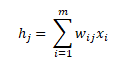

Backward Propagation: Update the weights using the following equation:

- Recall Phase: Compute the activation of the neuron j using the final weights using the following equations:
Backpropagation
It is a method for calculating the errors when values of Activation function and Target values mismatch. By using Backpropagation we will automatically update weights. For example:
- Consider output of Activation function is A(i) and Target Value is T(i)
- Calculate error between A and T, that is, ‘A(i) – T(i)’
- Let Input vector corresndin to above A(i) is x(k).
- Weighted Error W_error(k,i) = (A(i) – T(i)) * x(k)
- New_weight = Old_weight + (eta) * W_error
‘eta’ is the Learning Rate. It helps in controlling the rate of change in Weights. Sometimes the system gets unstable if weights change very rapidly and it never sets down, in such scenarios we use Learning Rate (eta). Typically we take eta as (0.1 < eta < 0.4).
Now whenever we get any kind of mismatch in the Activation and Target values, we do Backpropagation to update our weights.
Implementation of Perceptron
Creating of Input Matrix
In [49]:
import numpy as np

values=([2.7810836,2.550537003],
[1.465489372,	2.362125076],
[3.396561688,	4.400293529],
[1.38807019,1.850220317],
[3.06407232,3.005305973],
[7.627531214,	2.759262235],
[5.332441248,	2.088626775],
[6.922596716,	1.77106367],
[8.675418651,	-0.242068655],
[7.673756466,	3.508563011])

print("Training input values without Biasn", values)
Training input values without Bias
 ([2.7810836, 2.550537003], [1.465489372, 2.362125076], [3.396561688, 4.400293529], [1.38807019, 1.850220317], [3.06407232, 3.005305973], [7.627531214, 2.759262235], [5.332441248, 2.088626775], [6.922596716, 1.77106367], [8.675418651, -0.242068655], [7.673756466, 3.508563011])
Adding Bias to the Input Matrix
Bias value is like a cheat code to make training more reliable, now we will add biad value to Input matrix using ‘concatenate()’ method of numpy library.
In [50]:
test2 = [[-1]] * len(values)
values = np.concatenate((test2, values), axis = 1)
print("Training input values with bias in itn",values)
Training input values with bias in it
 [[-1.          2.7810836   2.550537  ]
 [-1.          1.46548937  2.36212508]
 [-1.          3.39656169  4.40029353]
 [-1.          1.38807019  1.85022032]
 [-1.          3.06407232  3.00530597]
 [-1.          7.62753121  2.75926224]
 [-1.          5.33244125  2.08862677]
 [-1.          6.92259672  1.77106367]
 [-1.          8.67541865 -0.24206865]
 [-1.          7.67375647  3.50856301]]
Creating Random Weights
We will generate random values of weights for Weight vector, using ‘rand()’ method of numpy library. Size of Weight vector will be equal to total number of values in a row of Input vector. In our case it is ‘3’, including bias value.
In [51]:
m=3     #number of elements in each row of inputs
n=1
weights = np.random.rand(m,n)*0.1 - 0.5
print("Initial random weightsn",weights)
Initial random weights
 [[-0.45303395]
 [-0.46630376]
 [-0.47939269]]
Target values Matrix
In [52]:
final = ([[0],[0],[0],[0],[0],[1],[1],[1],[1],[1]])
print("Training data target values aren", final)
Training data target values are
 [[0], [0], [0], [0], [0], [1], [1], [1], [1], [1]]
Method for updating Weights
If the value of Activation function is not equal to Target value, then we will use this method to update weights. We have introduced a new variable too, that is, Learning Rate (eta). It helps in controlling the rate of change in Weights. Sometimes the system gets unstable if weights change very rapidly and it never sets down, in such scenarios we use Learning Rate (eta). Typically we take eta as (0.1 < eta < 0.4). In our case we are taking it ‘0.25’
In [53]:
def updateWeights(weights, inputs, activation, targets):
    eta = 0.25
    weights += eta*np.dot(np.transpose(inputs), targets - activation)
    return weights
Creating method for Learning
This method calculates the Activation value and compares it with Target values, if they mismatch then the ‘updateWeights()’ method is being called to update weigts, then further Activation values are being calculated.
In [54]:
def  prediction (inputs, weights, targets):
    #representing Activation function with 'ack [[]]' variable
    ack = [[0]] * len(inputs)
    for i in range(0, len(inputs)):
        for j in range(0,len(weights)):
            ack[i] += inputs[i][j] * weights[j]
        ack[i] = np.where(ack[i]>0, 1, 0)
        #checking values with target
        if(targets[i] != ack[i]):
            weights = updateWeights(weights, inputs, ack[i], targets)
        print(ack[i])
    return weights
Training our model and extracting stable weights
Now we will do the training of our model, to do so we will use all the above data and methods and wil execute ‘prediction()’ method for ‘4’ times or until the Activation value gets equal to Target values and weights become stable.
In [55]:
iterations = 4
for temp in range(0, iterations):
    print("nIteration ",temp+1,"n")
    weights = prediction(values, weights, final)

print("nTrained Weightsn", weights)
Iteration  1

[0]
[0]
[0]
[0]
[0]
[0]
[1]
[1]
[1]
[1]

Iteration  2

[1]
[1]
[0]
[0]
[0]
[1]
[1]
[1]
[1]
[1]

Iteration  3

[0]
[0]
[0]
[0]
[0]
[1]
[1]
[1]
[1]
[1]

Iteration  4

[0]
[0]
[0]
[0]
[0]
[1]
[1]
[1]
[1]
[1]

Trained Weights
 [[ 0.79696605]
 [ 2.54399373]
 [-5.09227188]]
Testing our own data (Recall)
We will provide some data and our Perceptron will provide us some result corresponding to it. For this we will use Trained Weights that we extracted in above part and a new method ‘perceptronPredict()’
In [57]:
def perceptronPredict(weights, newInput):
    activation = np.dot(newInput, weights)
    activation = np.where(activation>0, 1, 0)
    print(activation)


newInput = ([-1.0, 1.786745, 2.94569],
            [-1.0, 7.023323, 1.9999])
perceptronPredict(weights, newInput)
Hence we got the results corresponding to each Input vector that we have supplied in the form of ‘newInput’ matrix.
Above post gave us an insight that how a basic Neural Network works and how it does the learning. In our next post we will learn a Multi-layer Neural Network!!
So stay tuned and keep learning!!!

Back To Top