В данной статье мы рассмотрим, что такое рекуррентные нейронные сети и как создать нейронную сеть с нуля в Python.
Содержание
- Зачем нужны рекуррентные нейронные сети
- Создание рекуррентной нейронной сети на примере
- Поставление задачи для рекуррентной нейронной сети
- Составление плана для нейронной сети
- Предварительная обработка рекуррентной нейронной сети RNN
- Фаза прямого распространения нейронной сети
- Фаза обратного распространения нейронной сети
- Параметры рассматриваемой нейронной сети
- Тестирование рекуррентной нейронной сети
Рекуррентные нейронные сети (RNN) — это тип нейронных сетей, которые специализируются на обработке последовательностей. Зачастую их используют в таких задачах, как обработка естественного языка (Natural Language Processing) из-за их эффективности в анализе текста. В данной статье мы наглядно рассмотрим рекуррентные нейронные сети, поймем принцип их работы, а также создадим одну сеть в Python, используя numpy.
Данная статья подразумевает наличие у читателя базовых знаний о нейронных сетях. Будет не лишним прочитать от том как создать нейронную сеть в Python, в которой показаны простые примеры использования нейронов в Python.
Приступим!
Зачем нужны рекуррентные нейронные сети
Один из нюансов работы с нейронными сетями (а также CNN) заключается в том, что они работают с предварительно заданными параметрами. Они принимают входные данные с фиксированными размерами и выводят результат, который также является фиксированным. Плюс рекуррентных нейронных сетей, или RNN, в том, что они обеспечивают последовательности с вариативными длинами как для входа, так и для вывода. Вот несколько примеров того, как может выглядеть рекуррентная нейронная сеть:
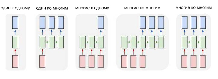
Входные данные отмечены красным, нейронная сеть RNN — зеленым, а вывод — синим.
Способность обрабатывать последовательности делает рекуррентные нейронные сети RNN весьма полезными. Области использования:
- Машинный перевод (пример Google Translate) выполняется при помощи нейронных сетей с принципом «многие ко многим». Оригинальная последовательность текста подается в рекуррентную нейронную сеть, которая затем создает переведенный текст в качестве результата вывода;
- Анализ настроений часто выполняется при помощи рекуррентных нейронных сетей с принципом «многие к одному». Этот отзыв положительный или отрицательный? Такая постановка является одним из примеров анализа настроений. Анализируемый текст подается нейронную сеть, которая затем создает единственную классификацию вывода. Например — Этот отзыв положительный.
Есть вопросы по Python?
На нашем форуме вы можете задать любой вопрос и получить ответ от всего нашего сообщества!
Telegram Чат & Канал
Вступите в наш дружный чат по Python и начните общение с единомышленниками! Станьте частью большого сообщества!
Паблик VK
Одно из самых больших сообществ по Python в социальной сети ВК. Видео уроки и книги для вас!
Далее в статье будет показан пример создания рекуррентной нейронной сети по схеме «многие к одному» для анализа настроений.
Создание рекуррентной нейронной сети на примере
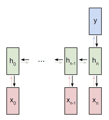
Представим, что у нас есть нейронная сеть, которая работает по принципу «многое ко многим«. Входные данные — x0, х1, … xn, а результаты вывода — y0, y1, … yn. Данные xi и yi являются векторами и могут быть произвольных размеров.
Рекуррентные нейронные сети RNN работают путем итерированного обновления скрытого состояния h, которое является вектором, что также может иметь произвольный размер. Стоит учитывать, что на любом заданном этапе t:
- Следующее скрытое состояние
htподсчитывается при помощи предыдущегоht - 1и следующим вводомxt; - Следующий вывод
ytподсчитывается при помощиht.
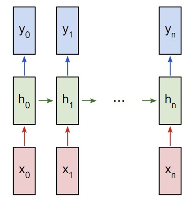 Рекуррентная нейронная сеть RNN многие ко многим
Вот что делает нейронную сеть рекуррентной: на каждом шаге она использует один и тот же вес. Говоря точнее, типичная классическая рекуррентная нейронная сеть использует только три набора параметров веса для выполнения требуемых подсчетов:
Wxhиспользуется для всех связокxt → htWhhиспользуется для всех связокht-1 → htWhyиспользуется для всех связокht → yt
Для рекуррентной нейронной сети мы также используем два смещения:
bhдобавляется при подсчетеhtbyдобавляется при подсчетеyt
Вес будет представлен как матрица, а смещение как вектор. В данном случае рекуррентная нейронная сеть состоит их трех параметров веса и двух смещений.
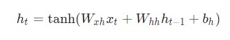
Следующие уравнения являются компактным представлением всего вышесказанного:
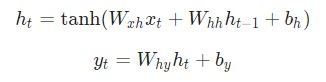
Разбор уравнений лучше не пропускать. Остановитесь на минутку и изучите их внимательно. Помните, что вес — это матрица, а другие переменные являются векторами.
Говоря о весе, мы используем матричное умножение, после чего векторы вносятся в конечный результат. Затем применяется гиперболическая функция в качестве функции активации первого уравнения. Стоит иметь в виду, что другие методы активации, например, сигмоиду, также можно использовать.
Не знаете, что такое функция активации? Вы можете ознакомиться с ними в вводной статье о нейронных сетях. Для оптимальной работы это важно.
Поставление задачи для рекуррентной нейронной сети
К текущему моменту мы смогли реализовать рекуррентную нейронную сеть RNN с нуля. Она должна выполнить простой анализ настроения. В дальнейшем примере мы попросим сеть определить, будет заданная строка нести позитивный или негативный характер.
Вот несколько примеров из небольшого набора данных, который был собран для данной статьи:
| Текст | Позитивный? |
| Я хороший | Да |
| Я плохой | Нет |
| Это очень хорошо | Да |
| Это неплохо | Да |
| Я плохой, а не хороший | Нет |
| Я несчастен | Нет |
| Это было хорошо | Да |
| Я чувствую себя неплохо, мне не грустно | Да |
Составление плана для нейронной сети
В следующем примере будет использована классификация рекуррентной сети «многие к одному». Принцип ее использования напоминает работу схемы «многие ко многим», что была описана ранее. Однако на этот раз будет задействовано только скрытое состояние для одного пункта вывода y:
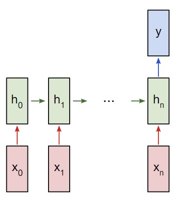
Рекуррентная нейронная сеть RNN многие к одному
Каждый xi будет вектором, представляющим определенное слово из текста. Вывод y будет вектором, содержащим два числа. Одно представляет позитивное настроение, а второе — негативное. Мы используем функцию Softmax, чтобы превратить эти значения в вероятности, и в конечном счете выберем между позитивным и негативным.
Приступим к созданию нашей рекуррентной нейронной сети.
Предварительная обработка рекуррентной нейронной сети RNN
Упомянутый ранее набор данных состоит из двух словарей Python:
|
train_data = { ‘good’: True, ‘bad’: False, # … больше данных } test_data = { ‘this is happy’: True, ‘i am good’: True, # … больше данных } |
True = Позитивное, False = Негативное
Для получения данных в удобном формате потребуется сделать определенную предварительную обработку. Для начала необходимо создать словарь в Python из всех слов, которые употребляются в наборе данных:
|
from data import train_data, test_data # Создание словаря vocab = list(set([w for text in train_data.keys() for w in text.split(‘ ‘)])) vocab_size = len(vocab) print(‘%d unique words found’ % vocab_size) # найдено 18 уникальных слов |
vocab теперь содержит список всех слов, которые употребляются как минимум в одном учебном тексте. Далее присвоим каждому слову из vocab индекс типа integer (целое число).
|
# Назначить индекс каждому слову word_to_idx = { w: i for i, w in enumerate(vocab) } idx_to_word = { i: w for i, w in enumerate(vocab) } print(word_to_idx[‘good’]) # 16 (это может измениться) print(idx_to_word[0]) # грустно (это может измениться) |
Теперь можно отобразить любое заданное слово при помощи индекса целого числа. Это очень важный пункт, так как:
Рекуррентная нейронная сеть не различает слов — только числа.
Напоследок напомним, что каждый ввод xi для рассматриваемой рекуррентной нейронной сети является вектором. Мы будем использовать веторы, которые представлены в виде унитарного кода. Единица в каждом векторе будет находиться в соответствующем целочисленном индексе слова.
Так как в словаре 18 уникальных слов, каждый xi будет 18-мерным унитарным вектором.
|
1 2 3 4 5 6 7 8 9 10 11 12 13 14 15 16 17 18 |
import numpy as np def createInputs(text): »’ Возвращает массив унитарных векторов которые представляют слова в введенной строке текста — текст является строкой string — унитарный вектор имеет форму (vocab_size, 1) »’ inputs = [] for w in text.split(‘ ‘): v = np.zeros((vocab_size, 1)) v[word_to_idx[w]] = 1 inputs.append(v) return inputs |
Мы используем createInputs() позже для создания входных данных в виде векторов и последующей их передачи в рекуррентную нейронную сеть RNN.
Фаза прямого распространения нейронной сети
Пришло время для создания рекуррентной нейронной сети. Начнем инициализацию с тремя параметрами веса и двумя смещениями.
|
import numpy as np from numpy.random import randn class RNN: # Классическая рекуррентная нейронная сеть def __init__(self, input_size, output_size, hidden_size=64): # Вес self.Whh = randn(hidden_size, hidden_size) / 1000 self.Wxh = randn(hidden_size, input_size) / 1000 self.Why = randn(output_size, hidden_size) / 1000 # Смещения self.bh = np.zeros((hidden_size, 1)) self.by = np.zeros((output_size, 1)) |
Обратите внимание: для того, чтобы убрать внутреннюю вариативность весов, мы делим на 1000. Это не самый лучший способ инициализации весов, но он довольно простой, подойдет для новичков и неплохо работает для данного примера.
Для инициализации веса из стандартного нормального распределения мы используем np.random.randn().
Затем мы реализуем прямую передачу рассматриваемой нейронной сети. Помните первые два уравнения, рассматриваемые ранее?
Эти же уравнения, реализованные в коде:
|
1 2 3 4 5 6 7 8 9 10 11 12 13 14 15 16 17 18 19 |
class RNN: # … def forward(self, inputs): »’ Выполнение передачи нейронной сети при помощи входных данных Возвращение результатов вывода и скрытого состояния Вывод — это массив одного унитарного вектора с формой (input_size, 1) »’ h = np.zeros((self.Whh.shape[0], 1)) # Выполнение каждого шага в нейронной сети RNN for i, x in enumerate(inputs): h = np.tanh(self.Wxh @ x + self.Whh @ h + self.bh) # Compute the output y = self.Why @ h + self.by return y, h |
Довольно просто, не так ли? Обратите внимание на то, что мы инициализировали h для нулевого вектора в первом шаге, так как у нас нет предыдущего h, который теперь можно использовать.
Давайте попробуем следующее:
|
# … def softmax(xs): # Применение функции Softmax для входного массива return np.exp(xs) / sum(np.exp(xs)) # Инициализация нашей рекуррентной нейронной сети RNN rnn = RNN(vocab_size, 2) inputs = createInputs(‘i am very good’) out, h = rnn.forward(inputs) probs = softmax(out) print(probs) # [[0.50000095], [0.49999905]] |
Наша рекуррентная нейронная сеть работает, однако ее с трудом можно назвать полезной. Давайте исправим этот недочет.
Фаза обратного распространения нейронной сети
Для тренировки рекуррентной нейронной сети будет использована функция потери. Здесь будет использована потеря перекрестной энтропии, которая в большинстве случаев совместима с функцией Softmax. Формула для подсчета:
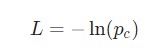
Здесь pc является предсказуемой вероятностью рекуррентной нейронной сети для класса correct (позитивный или негативный). Например, если позитивный текст предсказывается рекуррентной нейронной сетью как позитивный текст на 90%, то потеря составит:
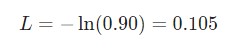
При наличии параметров потери можно натренировать нейронную сеть таким образом, чтобы она использовала градиентный спуск для минимизации потерь. Следовательно, здесь понадобятся градиенты.
Обратите внимание: следующий раздел подразумевает наличие у читателя базовых знаний об многовариантном исчислении. Вы можете пропустить несколько абзацев, однако мы рекомендуем все пробежаться по ним глазами. По мере получения новых данных код будет дополняться, и объяснения станут понятнее.
Оригиналы всех кодов, которые использованы в данной инструкции, доступны на GitHub.
Готовы? Продолжим!
Параметры рассматриваемой нейронной сети
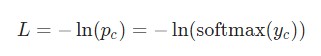
Параметры данных, которые будут использованы в дальнейшем:
y— необработанные входные данные нейронной сети;р— конечная вероятность:р = softmax(y);с— истинная метка определенного образца текста, так называемый «правильный» класс;L— потеря перекрестной энтропии:L = -ln(pc);Wxh,WhhиWhy— три матрицы веса в рассматриваемой нейронной сети;bhиby— два вектора смещения в рассматриваемой рекуррентной нейронной сети RNN.
Установка
Следующим шагом будет настройка фазы прямого распространения. Это необходимо для кеширования отдельных данных, которые будут использоваться в фазе обратного распространения нейронной сети. Параллельно с этим можно будет установить основной скелет для фазы обратного распространения. Это будет выглядеть следующим образом:
|
1 2 3 4 5 6 7 8 9 10 11 12 13 14 15 16 17 18 19 20 21 22 23 24 25 26 27 28 29 30 31 32 |
class RNN: # … def forward(self, inputs): »’ Выполнение фазы прямого распространения нейронной сети с использованием введенных данных. Возврат итоговой выдачи и скрытого состояния. — Входные данные в массиве однозначного вектора с формой (input_size, 1). »’ h = np.zeros((self.Whh.shape[0], 1)) self.last_inputs = inputs self.last_hs = { 0: h } # Выполнение каждого шага нейронной сети RNN for i, x in enumerate(inputs): h = np.tanh(self.Wxh @ x + self.Whh @ h + self.bh) self.last_hs[i + 1] = h # Подсчет вывода y = self.Why @ h + self.by return y, h def backprop(self, d_y, learn_rate=2e—2): »’ Выполнение фазы обратного распространения нейронной сети RNN. — d_y (dL/dy) имеет форму (output_size, 1). — learn_rate является вещественным числом float. »’ pass |
Градиенты
Настало время математики! Начнем с вычисления ![]() . Что нам известно:
. Что нам известно:
Здесь используется фактическое значение ![]() , а также применяется дифференцирование сложной функции. Результат следующий:
, а также применяется дифференцирование сложной функции. Результат следующий:
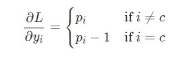
К примеру, если p = [0.2, 0.2, 0.6], а корректным классом является с = 0, то конечным результатом будет значение ![]()
= [-0.8, 0.2, 0.6]. Данное выражение несложно перевести в код:
|
# Цикл для каждого примера тренировки for x, y in train_data.items(): inputs = createInputs(x) target = int(y) # Прямое распространение out, _ = rnn.forward(inputs) probs = softmax(out) # Создание dL/dy d_L_d_y = probs d_L_d_y[target] -= 1 # Обратное распространение rnn.backprop(d_L_d_y) |
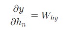
Отлично. Теперь разберемся с градиентами для Why и by, которые используются только для перехода конечного скрытого состояния в результат вывода рассматриваемой нейронной сети RNN. Используем следующие данные:
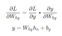
Здесь hn является конечным скрытым состоянием. Таким образом:
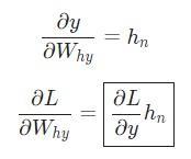
Аналогичным способом вычисляем:
Теперь можно приступить к реализации backprop().
|
class RNN: # … def backprop(self, d_y, learn_rate=2e—2): »’ Выполнение фазы обратного распространения нейронной сети RNN. — d_y (dL/dy) имеет форму (output_size, 1). — learn_rate является вещественным числом float. »’ n = len(self.last_inputs) # Подсчет dL/dWhy и dL/dby. d_Why = d_y @ self.last_hs[n].T d_by = d_y |
Напоминание: мы создали
self.last_hsвforward()в предыдущих примерах.
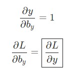
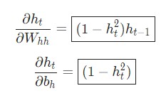
Наконец, нам понадобятся градиенты для Whh, Wxh, и bh, которые использовались в каждом шаге нейронной сети. У нас есть:
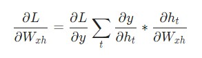
Изменение Wxh влияет не только на каждый ht, но и на все у , что, в свою очередь, приводит к изменениям в L. Для того, чтобы полностью подсчитать градиент Wxh, необходимо провести обратное распространение через все временные шаги. Его также называют Обратным распространением во времени, или Backpropagation Through Time (BPTT):
 Обратное распространение во времени
Wxh используется для всех прямых ссылок xt → ht, поэтому нам нужно провести обратное распространение назад к каждой из этих ссылок.
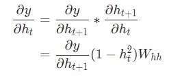
Приблизившись к заданному шагу t, потребуется подсчитать ![]() :
:
Производная гиперболической функции tanh нам уже известна:
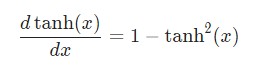
Используем дифференцирование сложной функции, или цепное правило:
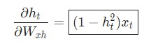
Аналогичным способом вычисляем:
Последнее нужное значение — ![]() . Его можно подсчитать рекурсивно:
. Его можно подсчитать рекурсивно:
Реализуем обратное распространение во времени, или BPTT, отталкиваясь от скрытого состояния в качестве начальной точки. Далее будем работать в обратном порядке. Поэтому на момент подсчета ![]() значение
значение ![]() будет известно. Исключением станет только последнее скрытое состояние
будет известно. Исключением станет только последнее скрытое состояние hn:
Теперь у нас есть все необходимое, чтобы наконец реализовать обратное распространение во времени ВРТТ и закончить backprop():
|
1 2 3 4 5 6 7 8 9 10 11 12 13 14 15 16 17 18 19 20 21 22 23 24 25 26 27 28 29 30 31 32 33 34 35 36 37 38 39 40 41 42 43 44 45 46 47 48 49 50 |
class RNN: # … def backprop(self, d_y, learn_rate=2e—2): »’ Выполнение фазы обратного распространения RNN. — d_y (dL/dy) имеет форму (output_size, 1). — learn_rate является вещественным числом float. »’ n = len(self.last_inputs) # Вычисление dL/dWhy и dL/dby. d_Why = d_y @ self.last_hs[n].T d_by = d_y # Инициализация dL/dWhh, dL/dWxh, и dL/dbh к нулю. d_Whh = np.zeros(self.Whh.shape) d_Wxh = np.zeros(self.Wxh.shape) d_bh = np.zeros(self.bh.shape) # Вычисление dL/dh для последнего h. d_h = self.Why.T @ d_y # Обратное распространение во времени. for t in reversed(range(n)): # Среднее значение: dL/dh * (1 — h^2) temp = ((1 — self.last_hs[t + 1] ** 2) * d_h) # dL/db = dL/dh * (1 — h^2) d_bh += temp # dL/dWhh = dL/dh * (1 — h^2) * h_{t-1} d_Whh += temp @ self.last_hs[t].T # dL/dWxh = dL/dh * (1 — h^2) * x d_Wxh += temp @ self.last_inputs[t].T # Далее dL/dh = dL/dh * (1 — h^2) * Whh d_h = self.Whh @ temp # Отсекаем, чтобы предотвратить разрыв градиентов. for d in [d_Wxh, d_Whh, d_Why, d_bh, d_by]: np.clip(d, —1, 1, out=d) # Обновляем вес и смещение с использованием градиентного спуска. self.Whh -= learn_rate * d_Whh self.Wxh -= learn_rate * d_Wxh self.Why -= learn_rate * d_Why self.bh -= learn_rate * d_bh self.by -= learn_rate * d_by |
Моменты, на которые стоит обратить внимание:
Мы сделали это! Наша рекуррентная нейронная сеть готова.
Тестирование рекуррентной нейронной сети
Наконец настал тот момент, которого мы так долго ждали — протестируем готовую рекуррентную нейронную сеть.
Для начала, напишем вспомогательную функцию для обработки данных рассматриваемой рекуррентной нейронной сети:
|
1 2 3 4 5 6 7 8 9 10 11 12 13 14 15 16 17 18 19 20 21 22 23 24 25 26 27 28 29 30 31 32 33 34 35 36 |
import random def processData(data, backprop=True): »’ Возврат потери рекуррентной нейронной сети и точности для данных — данные представлены как словарь, что отображает текст как True или False. — backprop определяет, нужно ли использовать обратное распределение »’ items = list(data.items()) random.shuffle(items) loss = 0 num_correct = 0 for x, y in items: inputs = createInputs(x) target = int(y) # Прямое распределение out, _ = rnn.forward(inputs) probs = softmax(out) # Вычисление потери / точности loss -= np.log(probs[target]) num_correct += int(np.argmax(probs) == target) if backprop: # Создание dL/dy d_L_d_y = probs d_L_d_y[target] -= 1 # Обратное распределение rnn.backprop(d_L_d_y) return loss / len(data), num_correct / len(data) |
Теперь можно написать цикл для тренировки сети:
|
# Цикл тренировки for epoch in range(1000): train_loss, train_acc = processData(train_data) if epoch % 100 == 99: print(‘— Epoch %d’ % (epoch + 1)) print(‘Train:tLoss %.3f | Accuracy: %.3f’ % (train_loss, train_acc)) test_loss, test_acc = processData(test_data, backprop=False) print(‘Test:tLoss %.3f | Accuracy: %.3f’ % (test_loss, test_acc)) |
Результат вывода main.py выглядит следующим образом:
|
1 2 3 4 5 6 7 8 9 10 11 12 13 14 15 16 17 18 19 20 21 22 23 24 25 26 27 28 29 30 |
—— Epoch 100 Train: Loss 0.688 | Accuracy: 0.517 Test: Loss 0.700 | Accuracy: 0.500 —— Epoch 200 Train: Loss 0.680 | Accuracy: 0.552 Test: Loss 0.717 | Accuracy: 0.450 —— Epoch 300 Train: Loss 0.593 | Accuracy: 0.655 Test: Loss 0.657 | Accuracy: 0.650 —— Epoch 400 Train: Loss 0.401 | Accuracy: 0.810 Test: Loss 0.689 | Accuracy: 0.650 —— Epoch 500 Train: Loss 0.312 | Accuracy: 0.862 Test: Loss 0.693 | Accuracy: 0.550 —— Epoch 600 Train: Loss 0.148 | Accuracy: 0.914 Test: Loss 0.404 | Accuracy: 0.800 —— Epoch 700 Train: Loss 0.008 | Accuracy: 1.000 Test: Loss 0.016 | Accuracy: 1.000 —— Epoch 800 Train: Loss 0.004 | Accuracy: 1.000 Test: Loss 0.007 | Accuracy: 1.000 —— Epoch 900 Train: Loss 0.002 | Accuracy: 1.000 Test: Loss 0.004 | Accuracy: 1.000 —— Epoch 1000 Train: Loss 0.002 | Accuracy: 1.000 Test: Loss 0.003 | Accuracy: 1.000 |
Неплохо для рекуррентной нейронной сети, которую мы построили сами!
Хотите поэкспериментировать с этим кодом сами? Можете запустить данную рекуррентную нейронную сеть RNN у себя в браузере. Она также доступна на GitHub.
Подведем итоги
Вот и все, пошаговое руководство по рекуррентным нейронным сетям на этом закончено. Мы узнали, что такое RNN, как они работают, почему они полезны, как их создавать и тренировать. Это очень малый аспект мира нейронных сетей. При желании вы можете продолжить изучение темы самостоятельно, используя следующие ресурсы:
- Подробнее ознакомьтесь с LTSM. Это долгая краткосрочная память, которая характерна более мощной архитектурой рекуррентных нейронных сетей. Будет не лишним ознакомиться с управляемым рекуррентными блоками, или GRU. Это наиболее популярная вариация LTSM;
- Поэкспериментируйте с более крупными и сложными RNN. Для этого используйте подходящие ML библиотеки, например, Tensorflow, Keras или PyTorch;
- Прочтите о двунаправленных нейронных сетях, которые обрабатывают последовательности как в прямом, так и в обратном направлении. Это позволяет получить больше информации на уровне вывода;
- Ознакомьтесь с векторными представлением слов. Для этого можно использовать GloVe или Word2Vec;
- Познакомьтесь поближе с Natural Language Toolkit (NLTK), популярной библиотекой Python для работы с данными на языках, которые используют люди, а не машины.
Благодарим за внимание!

Являюсь администратором нескольких порталов по обучению языков программирования Python, Golang и Kotlin. В составе небольшой команды единомышленников, мы занимаемся популяризацией языков программирования на русскоязычную аудиторию. Большая часть статей была адаптирована нами на русский язык и распространяется бесплатно.
E-mail: vasile.buldumac@ati.utm.md
Образование
Universitatea Tehnică a Moldovei (utm.md)
- 2014 — 2018 Технический Университет Молдовы, ИТ-Инженер. Тема дипломной работы «Автоматизация покупки и продажи криптовалюты используя технический анализ»
- 2018 — 2020 Технический Университет Молдовы, Магистр, Магистерская диссертация «Идентификация человека в киберпространстве по фотографии лица»
N+1 совместно с МФТИ продолжает знакомить читателя с наиболее яркими аспектами современных исследований в области искусственного интеллекта. В прошлый раз мы писали об общих принципах машинного обучения и конкретно о методе обратного распространения ошибки для обучения нейросетей. Сегодня наш собеседник — Валентин Малых, младший научный сотрудник Лаборатории нейронных систем и глубокого обучения. Вместе с ним мы поговорим о необычном классе этих систем — рекуррентных нейросетях, их особенностях и перспективах, как на поприще всевозможных развлечений в стиле DeepDream, так и в «полезных» областях. Поехали.
Что такое рекуррентные нейросети (РНС) и чем они отличаются от обычных?
Давайте сначала вспомним, что такое «обычные» нейросети, и тогда сразу станет понятно, чем они отличаются от реккурентных. Представим себе самую простую нейросеть — перцептрон. Он представляет собой один слой нейронов, каждый из которых принимает кусочек входных данных (один или несколько битов, действительных чисел, пикселей и т.п.), модифицирует его с учетом собственного веса и передает дальше. В однослойном перцептроне выдача всех нейронов объединяется тем или иным образом, и нейросеть дает ответ, но возможности такой архитектуры сильно ограниченны. Если вы хотите получить более продвинутый функционал, можно пойти несколькими путями, например, увеличить количество слоев и добавить операцию свертки, которая бы «расслаивала» входящие данные на кусочки разных масштабов. В этом случае у вас получатся сверточные нейросети для глубинного обучения, которые преуспели в обработке изображений и распознавании котиков. Однако что у примитивного перцептрона, что у сверточной нейросети есть общее ограничение: и входные и выходные данные имеют фиксированный, заранее обозначенный размер, например, картинка 100×100 пикселей или последовательность из 256 бит. Нейросеть с математической точки зрения ведет себя как обычная функция, хоть и очень сложно устроенная: у нее есть заранее обозначенное число аргументов, а также обозначенный формат, в котором она выдает ответ. Простой пример — функция x2, она принимает один аргумент и выдает одно значение.
Вышеперечисленные особенности не представляет больших трудностей, если речь идет о тех же картинках или заранее определенных последовательностях символов. Но что, если вы хотите использовать нейросеть для обработки текста или музыки? В общем случае — любой условно бесконечной последовательности, в которой важно не только содержание, но и порядок, в котором следует информация. Вот для этих задач и были придуманы рекуррентные нейросети. Их противоположности, которые мы называли «обычными», имеют более строгое название — нейросети прямого распространения (feed-forward neural networks), так как в них информация передается только вперед по сети, от слоя к слою. В рекуррентных нейросетях нейроны обмениваются информацией между собой: например, вдобавок к новому кусочку входящих данных нейрон также получает некоторую информацию о предыдущем состоянии сети. Таким образом в сети реализуется «память», что принципиально меняет характер ее работы и позволяет анализировать любые последовательности данных, в которых важно, в каком порядке идут значения — от звукозаписей до котировок акций.
Наличие памяти у рекуррентных нейросетей позволяет несколько расширить нашу аналогию с x
2
. Если нейросети прямого распространения мы назвали «простой» функцией, то рекуррентные нейросети можно почти с чистой совестью назвать программой. В самом деле, память рекуррентных нейросетей (хотя и не полноценная, но об этом позже) делает их Тьюринг-полными: при правильном задании весов нейросеть может успешно эмулировать работу компьютерных программ.
Немного углубимся в историю: когда были придуманы РНС, для каких задач и в чем, как тогда казалось, должно было заключаться их преимущество перед обычным перцептроном?
Вероятно, первой РНС была сеть Хопфилда (впервые упомянута в 1974 году, окончательно оформилась в 1982-м), которая реализовывала на практике ячейку ассоциативной памяти. От современных РНС она отличается тем, что работает с последовательностями фиксированного размера. В простейшем случае сеть Хопфилда имеет один слой внутренних нейронов, связанных между собой, а каждая связь характеризуется определенным весом, задающим ее значимость. С такой сетью ассоциируется некий эквивалент физической «энергии», который зависит от всех весов в системе. Сеть можно обучить при помощи градиентного спуска по энергии, когда минимум соответствует состоянию, в котором сеть «запомнила» определенный шаблон, например 10101. Теперь, если ей на вход подать искаженный, зашумленный или неполный шаблон, скажем, 10000, она «вспомнит» и восстановит его аналогично тому, как работает ассоциативная память у человека. Эта аналогия достаточно отдаленна, поэтому не стоит воспринимать ее чересчур серьезно. Тем не менее, сети Хопфилда успешно справлялись со своей задачей и обходили по возможностям существовавшие тогда перцептроны. Интересно, что оригинальная публикация Джона Хопфилда в Proceedings of the National Academy of Sciences вышла в разделе «Биофизика».
Следующим шагом в эволюции РНС была
Джеффа Элмана, описанная в 1990 году. В ней автор подробно затронул вопрос о том, как можно (и можно ли вообще) обучить нейросеть распознавать временные последовательности. Например, если есть входящие данные
1100
и
0110
, можно ли их считать одним и тем же набором, сдвинутым во времени? Конечно, можно, но как обучить этому нейросеть? Обычный перцептрон легко запомнит эту закономерность для любых примеров, которые ему предложат, но каждый раз это будет задачей сравнения двух разных сигналов, а не задачей об эволюции или сдвиге одного и того же сигнала. Решение Элмана, основанное на предыдущих наработках в этой области, основывалось на том, что в простую нейросеть добавлялся еще один — «контекстный» — слой, в который просто копировалось состояние внутреннего слоя нейронов на каждом цикле работы сети. При этом связь между контекстным и внутренним слоями можно было обучать. Такая архитектура позволяла сравнительно легко воспроизводить временные ряды, а также обрабатывать последовательности произвольной длины, что резко отличало простую РНС Элмана от предыдущих концепций. Более того, эта сеть смогла распознать и даже классифицировать существительные и глаголы в предложении, основываясь только на порядке слов, что было настоящим прорывом для своего времени и вызвало огромный интерес как лингвистов, так и специалистов по исследованию сознания.
За простой РНС Элмана последовали все новые разработки, а в 1997 году Хохрейтер и Шмидхубер опубликовали статью «
» («долгосрочная краткосрочная память», также существует множество других вариаций перевода), заложившую основу для большинства современных РНС. В своей работе авторы описывали модификацию, решавшую проблему долгосрочной памяти простых РНС: их нейроны хорошо «помнят» недавно полученную информацию, но не имеют возможности надолго сохранить в памяти что-то, что обработали много циклов назад, какой бы важной та информация ни была. В LSTM-сетях внутренние нейроны «оборудованы» сложной системой так называемых ворот (gates), а также концепцией клеточного состояния (cell state), которая и представляет собой некий вид долгосрочной памяти. Ворота же определяют, какая информация попадет в клеточное состояние, какая сотрется из него, и какая повлияет на результат, который выдаст РНС на данном шаге. Подробно разбирать LSTM мы не будем, однако отметим, что именно эти вариации РНС широко используется сейчас, например, для машинного перевода Google.
Все прекрасно звучит на словах, но что все-таки РНС умеют делать? Вот дали им текст почитать или музыку послушать — а дальше что?
Одна из главных областей применения РНС на сегодняшний день — работа с языковыми моделями, в частности — анализ контекста и общей связи слов в тексте. Для РНС структура языка — это долгосрочная информация, которую надо запомнить. К ней относятся грамматика, а также стилистические особенности того корпуса текстов, на которых производится обучение. Фактически РНС запоминает, в каком порядке обычно следуют слова, и может дописать предложение, получив некоторую затравку. Если эта затравка случайная, может получиться совершенно бессмысленный текст, стилистически напоминающий шаблон, на котором училась РНС. Если же исходный текст был осмысленным, РНС поможет его стилизовать, однако в последнем случае одной РНС будет мало, так как результат должен представлять собой «смесь» случайного, но стилизованного текста от РНС и осмысленной, но «неокрашенной» исходной части. Эта задача уже настолько напоминает популярные ныне
для обработки фотографий в стиле Моне и Ван Гога, что невольно напрашивается аналогия.
Действительно, задача переноса стиля с одного изображения на другой решается при помощи нейросетей и операции свертки, которая разбивает изображение на несколько масштабов и позволяет нейросетям анализировать их независимо друг от друга, а впоследствии и перемешивать между собой. Аналогичные операции
и с музыкой (также с помощью сверточных нейросетей): в этом случае мелодия является содержанием, а аранжировка — стилем. И вот с написанием музыки РНС как раз успешно
. Поскольку обе задачи — и написание, и смешивание мелодии с произвольным стилем — уже успешно решены при помощи нейросетей, совместить эти решения остается делом техники.
Наконец, давайте разберемся, почему музыку РНС худо-бедно пишут, а с полноценными текстами Толстого и Достоевского возникают проблемы? Дело в том, что в инструментальной музыке, как бы по-варварски это ни звучало, нет
смысла
в том же значении, в каком он есть в большинстве текстов. То есть музыка может нравиться или не нравиться, но если в ней нет слов — она не несет информационной нагрузки (конечно, если это не секретный код). Именно с приданием своим произведениям смысла и наблюдаются проблемы у РНС: они могут превосходно выучить грамматику языка и запомнить, как должен
выглядеть
текст в определенном стиле, но создать и донести какую-то идею или информацию РНС (пока) не могут.
Особый случай в этом вопросе — это автоматическое написание программного кода. Действительно, поскольку язык программирования по определению представляет собой
язык
, РНС может его выучить. На практике оказывается, что программы, написанные РНС, вполне успешно компилируются и запускаются, однако они не делают ничего полезного, если им заранее не
. А причина этого та же, что и в случае литературных текстов: для РНС язык программирования — не более чем стилизация, в которую они, к сожалению, не могут вложить никакого смысла.
«Генерация бреда» это забавно, но бессмысленно, а для каких настоящих задач применяются РНС?
Разумеется, РНС, помимо развлекательных, должны преследовать и более прагматичные цели. Из их дизайна автоматически следует, что главные области их применения должны быть требовательны к контексту и/или временной зависимости в данных, что по сути одно и то же. Поэтому РНС используются, к примеру, для анализа изображений. Казалось бы, эта область обычно воспринимается в контексте сверточных нейросетей, однако и для РНС здесь находятся задачи: их архитектура позволяет быстрее распознавать детали, основываясь на контексте и окружении. Аналогичным образом РНС работают в сферах анализа и генерации текстов. Из более необычных задач можно
попытки использовать ранние РНС для классификации углеродных спектров ядерного магнитного резонанса различных производных бензола, а из современных — анализ появления негативных отзывов о товарах.
А каковы успехи РНС в машинном переводе? В Google Translate ведь именно они используются?
На текущий момент в Google для машинного перевода
РНС типа LSTM, что позволило добиться наибольшей точности по сравнению с существующими аналогами, однако, по словам самих авторов, машинному переводу еще очень далеко до уровня человека. Сложности, с которыми сталкиваются нейросети в задачах перевода, обусловлены сразу несколькими факторами: во-первых, в любой задаче существует неизбежный размен между качеством и скоростью. На данный момент человек очень сильно опережает искусственный интеллект по этому показателю. Поскольку машинный перевод чаще всего используется в онлайн-сервисах, разработчики вынуждены жертвовать точностью в угоду быстродействию. В недавней публикации Google на эту тему разработчики подробно описывают многие решения, которые позволили оптимизировать текущую версию Google Translate, однако проблема до сих пор остается. Например, редкие слова, или сленг, или нарочитое искажение слова (например, для более яркого заголовка) может сбить с толку даже переводчика-человека, которому придется потратить время, чтобы подобрать наиболее адекватный аналог в другом языке. Машину же такая ситуация поставит в полный тупик, и переводчик будет вынужден «выбросить» сложное слово и оставить его без перевода. В итоге проблема машинного перевода не настолько обусловлена архитектурой (РНС успешно справляются с рутинными задачами в этой области), насколько сложностью и многообразием языка. Радует то, что эта проблема имеет более технический характер, чем написание осмысленных текстов, где, вероятно, требуется кардинально новый подход.
А более необычные способы применения РНС есть? Вот нейронная машина Тьюринга, например, в чем тут идея?
Нейронная машина Тьюринга (
), предложенная два года назад коллективом из Google DeepMind, отличается от других РНС тем, что последние на самом деле не хранят информацию в явном виде — она кодируется в весах нейронов и связей, даже в продвинутых вариациях вроде LSTM. В нейронной машине Тьюринга разработчики придерживались более понятной идеи «ленты памяти», как в классической машине Тьюринга: в ней информация в явном виде записывается «на ленту» и может быть считана в случае необходимости. При этом отслеживание того, какая информация нужна, ложится на особую нейросеть-контроллер. В целом можно отметить, что идея НМТ действительно завораживает своей простотой и доступностью для понимания. С другой стороны, в силу технических ограничений современного аппаратного обеспечения применить НМТ на практике не представляется возможным, потому что обучение такой сети становится чрезвычайно долгим. В этом смысле РНС являются промежуточным звеном между более простыми нейросетями и НМТ, так как хранят некий «слепок» информации, который при этом не смертельно ограничивает их быстродействие.
А что такое концепция внимания применительно к РНС? Что нового она позволяет делать?
Концепция внимания (attention) — это способ «подсказать» сети, на что следует потратить больше внимания при обработке данных. Другими словами, внимание в рекуррентной нейронной сети — это способ увеличить важность одних данных по сравнению с другими. Поскольку человек не может выдавать подсказки каждый раз (это нивелировало бы всю пользу от РНС), сеть должна научиться подсказывать себе сама. Вообще, концепция внимания является очень сильным инструментом в работе с РНС, так как позволяет быстрее и качественнее подсказать сети, на какие данные стоит обращать внимание, а на какие — нет. Также этот подход может в перспективе решить проблему быстродействия в системах с большим объемом памяти. Чтобы лучше понять, как это работает, надо рассмотреть две модели внимания: «мягкую» (soft) и «жесткую» (hard). В первом случае сеть все равно обратится ко всем данным, к которым имеет доступ, но значимость (то есть вес) этих данных будет разной. Это делает РНС более точной, но не более быстрой. Во втором случае из всех существующих данных сеть обратится лишь к некоторым (у остальных будут нулевые веса), что решает сразу две проблемы. Минусом «жесткой» концепции внимания является тот факт, что эта модель перестает быть непрерывной, а значит — дифференцируемой, что резко усложняет задачу ее обучения. Тем не менее, существуют решения, позволяющие исправить этот недостаток. Поскольку концепция внимания активно развивается в последние пару лет, нам остается ждать в ближайшее время новостей с этого поля.
Под конец можно привести пример системы, использующей концепцию внимания: это Dynamic Memory Networks — разновидность, предложенная исследовательским подразделением Facebook. В ней разработчики описывают «модуль эпизодической памяти» (episodic memory module), который на основании памяти о событиях, заданных в виде входных данных, а также вопроса об этих событиях, создает «эпизоды», которые в итоге помогают сети найти правильный ответ на вопрос. Такая архитектура была опробована на bAbI, крупной базе сгенерированных заданий на простой логический вывод (например, дается цепочка из трех фактов, нужно выдать правильный ответ: «Мэри дома. Она вышла во двор. Где Мэри? Во дворе».), и показала результаты, превосходящие классические архитектуры вроде LSTM.
Что еще происходит в мире рекуррентных нейросетей прямо сейчас?
По словам Андрея Карпатого (Andrej Karpathy) — специалиста по нейросетям и автора превосходного блога, «концепция внимания — это самое интересное из недавних архитектурных решений в мире нейросетей». Однако не только на внимании акцентируются исследования в области РНС. Если постараться кратко сформулировать основной тренд, то им сейчас стало сочетание различных архитектур и применение наработок из других областей для улучшения РНС. Из примеров можно назвать уже упомянутые нейросети от Google, в которых используют методы, взятые из работ по обучению с подкреплением, нейронные машины Тьюринга, алгоритмы оптимизации вроде Batch Normalization и многое другое, — все это вместе заслуживает отдельной статьи. В целом отметим, что хотя РНС не привлекли столь же широкого внимания, как любимцы публики — сверточные нейросети, это объясняется лишь тем, что объекты и задачи, с которыми работают РНС, не так бросаются в глаза, как DeepDream или Prisma. Это как в социальных сетях — если пост публикуют без картинки, ажиотажа вокруг него будет меньше.
Поэтому всегда публикуйтесь с картинкой.
Тарас Молотилин
Перевод
Ссылка на автора
Основная цель этого поста — внедрить RNN с нуля и дать простое объяснение, чтобы сделать его полезным для читателей. Внедрение любой нейронной сети с нуля хотя бы один раз является ценным упражнением. Это поможет вам понять, как работают нейронные сети, и здесь мы внедряем RNN, который имеет свою сложность и, таким образом, дает нам хорошую возможность отточить наши навыки.

Существуют различные учебные пособия, которые предоставляют очень подробную информацию о внутренностях RNN. Вы можете найти некоторые из очень полезных ссылок в конце этого поста. Я довольно быстро понял, как работает RNN, но больше всего меня беспокоило то, как проходили расчеты BPTT и их реализация. Мне пришлось потратить некоторое время, чтобы понять и, наконец, собрать все вместе. Не теряя больше времени, давайте сначала быстро пройдемся по основам RNN.
Что такое RNN?
Рекуррентная нейронная сеть — это нейронная сеть, которая специализируется на обработке последовательности данных.x(t)= x(1), . . . , x(τ)с индексом временного шагаtначиная от1 to τ, Для задач, которые включают последовательные вводы, такие как речь и язык, часто лучше использовать RNN. В задаче НЛП, если вы хотите предсказать следующее слово в предложении, важно знать слова перед ним. RNNs называютсявозвратныйпотому что они выполняют одну и ту же задачу для каждого элемента последовательности с выходом, зависящим от предыдущих вычислений. Еще один способ думать о RNN — это то, что у них есть «память», которая собирает информацию о том, что было рассчитано до сих пор.
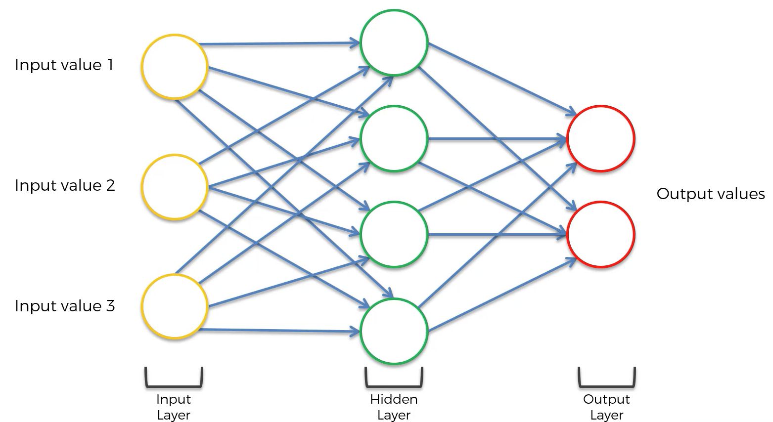
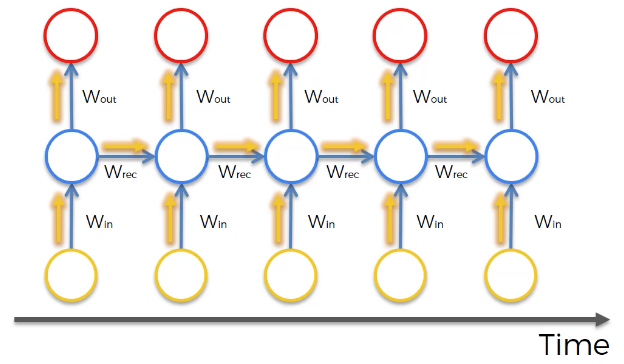
Архитектура:Давайте кратко пройдемся по базовой сети RNN.

Левая сторона вышеприведенной диаграммы показывает обозначение RNN, а справа — RNN.развернутый(или развернутый) в полную сеть. Развертывание означает, что мы выписываем сеть для полной последовательности. Например, если интересующая нас последовательность представляет собой предложение из трех слов, сеть будет развернута в трехслойную нейронную сеть, по одному слою для каждого слова.
Входные данные:х (т)Принимается за вход в сеть на шаге по временит.Например,x1,может быть горячим вектором, соответствующим слову предложения.
Скрытое состояние: ч (т)Представляет скрытое состояние в момент времени t и действует как «память» сети.ч (т)Рассчитывается на основе текущего ввода и скрытого состояния предыдущего временного шага:h(t) = f(U x(t) + W h(t−1)).Функцияfпринимается за нелинейное преобразование, такое какTANH,РЕЛУ.
Веса: RNN имеет вход для скрытых соединений, параметризованных весовой матрицей U, скрытых к скрытым рекуррентным соединениям, параметризованным весовой матрицей W, и скрытых к выходу соединений, параметризованных весовой матрицей V и всеми этими весами (U,В,W)распределяются по времени.
Выход:о (т)Иллюстрирует вывод сети. На рисунке я просто поместил стрелку послео (т)который также часто подвергается нелинейности, особенно когда сеть содержит дополнительные уровни ниже по потоку.
Форвард Пасс
На рисунке не указан выбор функции активации для скрытых юнитов. Прежде чем продолжить, сделаем несколько предположений: 1) мы предполагаем гиперболическую касательную функцию активации для скрытого слоя. 2) Мы предполагаем, что выходные данные являются дискретными, как будто RNN используется для предсказания слов или символов. Естественным способом представления дискретных переменных является учет выходных данных.oкак предоставление ненормированных логарифмических вероятностей каждого возможного значения дискретной переменной. Затем мы можем применить операцию softmax в качестве шага постобработки, чтобы получить векторŷнормированных вероятностей на выходе.
Прямой проход RNN, таким образом, может быть представлен нижеследующей системой уравнений.

Это пример рекуррентной сети, которая отображает входную последовательность на выходную последовательность той же длины. Общая потеря для данной последовательностиxзначения в паре с последовательностьюyЗначения тогда будут просто суммой потерь за все временные шаги. Мы предполагаем, что выводыo(t)используются в качестве аргумента функции softmax для получения вектораŷвероятностей на выходе. Мы также предполагаем, что потеряLотрицательная логарифмическая вероятность истинной целиy(t)учитывая вклад до сих пор.
Обратный проход
Вычисление градиента включает выполнение прохода прямого распространения, перемещающегося слева направо по графику, показанному выше, за которым следует проход обратного распространения, перемещающийся справа налево по графику. Время выполнения равно O (τ) и не может быть уменьшено путем распараллеливания, поскольку граф прямого распространения по своей природе является последовательным; каждый временной шаг может быть вычислен только после предыдущего. Состояния, вычисленные в прямом проходе, должны храниться до их повторного использования во время обратного прохода, поэтому стоимость памяти также равна O (τ) Алгоритм обратного распространения, применяемый к развернутому графу со стоимостью O (τ), называется обратным распространением во времени (BPTT). Поскольку параметры являются общими для всех временных шагов в сети, градиент на каждом выходе зависит не только от вычислений текущего временного шага, но и от предыдущих временных шагов.
Вычислительные градиенты
Учитывая нашу функцию потерьLнам нужно вычислить градиенты для наших трех весовых матрицU, V, W иусловия смещенияДо нашей эрыи обновить ихсо скоростью обученияα, Подобно нормальному обратному распространению, градиент дает нам представление о том, как изменяется потеря по отношению к каждому весовому параметру. Мы обновляем веса W, чтобы минимизировать потери с помощью следующего уравнения:

То же самое должно быть сделано и для других весов U, V, b, c.
Давайте теперь вычислим градиенты по BPTT для приведенных выше уравнений RNN. Узлы нашего вычислительного графа включают в себя параметры U, V, W, b и c, а также последовательность узлов, индексированных t для x (t), h (t), o (t) и L (t). Для каждого узлаnнам нужно вычислить градиент∇nLрекурсивно, на основе градиента, вычисленного в узлах, следующих за ним в графе.
Градиент по выходу o (t)рассчитывается при условии, что o (t) используются в качестве аргумента функции softmax для получения вектораŷвероятностей на выходе. Мы также предполагаем, что потеря является отрицательной логарифмической вероятностью истинной цели y (t).

Пожалуйста, обратитесь Вот для получения вышеуказанного элегантного решения.
Давайте теперь разберемся, как градиент течет через скрытое состояние h (t). Это ясно видно из диаграммы ниже, что в момент времени t скрытое состояние h (t) имеет градиент, вытекающий как из токового выхода, так и из следующего скрытого состояния.

Мы работаем в обратном направлении, начиная с конца последовательности. На конечном шаге по времени τ h (τ) имеет только o (τ) в качестве потомка, поэтому его градиент прост:

Затем мы можем выполнить итерацию назад во времени для обратного распространения градиентов во времени, от t = τ − 1 до t = 1, отметив, что h (t) (для t <τ) имеет в качестве потомков o (t) и h ( T + 1). Таким образом, его градиент определяется как:

Как только градиенты на внутренних узлах вычислительного графа получены, мы можем получить градиенты на узлах параметров. Расчет градиента с использованием правила цепочки для всех параметров:

Мы не заинтересованы выводить эти уравнения здесь, а реализуем их. Там очень хорошие посты Вот а также Вот предоставляя подробный вывод этих уравнений.
Реализация
Мы реализуем полную Рекуррентную Нейронную Сеть с нуля, используя Python. Мы попытаемся построить модель генерации текста с использованием RNN. Мы обучаем нашу модель прогнозированию вероятности персонажа с учетом предыдущих символов. Этогенеративная модель, Учитывая существующую последовательность символов, мы выбираем следующий символ из предсказанных вероятностей и повторяем процесс, пока у нас не будет полного предложения. Эта реализация от Андрея Карпарти отличный пост построение уровня персонажа RNN. Здесь мы обсудим детали реализации шаг за шагом.
Общие шаги, чтобы следовать:
- Инициализировать весовые матрицыU, V, Wот случайного распределенияи смещение b, c с нулями
- Прямое распространение для вычисления прогнозов
- Вычислить потери
- Обратное распространение для вычисления градиентов
- Обновление весов на основе градиентов
- Повторите шаги 2–5
Шаг 1: Инициализация
Чтобы начать с реализации базовой ячейки RNN, мы сначала определим размеры различных параметров U, V, W, b, c.
Размеры: Допустим, мы выбрали размер словаряvocab_size= 8000и скрытый размер слояhidden_size=100, Тогда мы имеем:

Размер словаря может быть числом уникальных символов для модели на основе символов или количеством уникальных слов для модели на основе слов.
С нашими немногими гиперпараметрами и другими параметрами модели давайте начнем определять нашу ячейку RNN.

Правильная инициализация весов, похоже, влияет на результаты тренировок, в этой области было проведено много исследований. Оказывается, что лучшая инициализация зависит от функции активации (в нашем случае tanh) и одной рекомендуемые подход состоит в том, чтобы инициализировать веса случайным образом в интервале от[ -1/sqrt(n), 1/sqrt(n)]гдеnэто количество входящих соединений с предыдущего слоя.
Шаг 2: прямой проход
В соответствии с нашими уравнениями для каждой временной метки t мы вычисляем скрытое состояние hs [t] и выводим os [t], применяя softmax, чтобы получить вероятность для следующего символа.

Вычисление softmax и численная стабильность:
Функция Softmax берет N-мерный вектор действительных чисел и преобразует его в вектор действительного числа в диапазоне (0,1), который складывается в 1. Отображение выполняется с использованием приведенной ниже формулы

Реализация softmax это:


Хотя это выглядит хорошо, однако, когда мы называем это softmax с большим числом, как показано ниже, это дает значения «nan»

Числовой диапазон чисел с плавающей точкой, используемых Numpy, ограничен. Для float64 максимальное представляемое число порядка 10³⁰⁸. Экспонирование в функции softmax позволяет легко сбросить это число, даже для входов довольно скромного размера. Хороший способ избежать этой проблемы — нормализовать входные данные, чтобы они не были слишком большими или слишком маленькими. Существует небольшой математический трюк Вот для деталей. Итак, наш софтмакс выглядит так:

Шаг 3: вычислить потери
Поскольку мы реализуем модель генерации текста, следующим символом может быть любой из уникальных символов в нашем словаре. Таким образом, наша потеря будет кросс-энтропийной потерей. В мультиклассовой классификации мы берем сумму значений логарифмических потерь для каждого прогноза класса в наблюдении.

- M — количество возможных меток классов (уникальные символы в нашем словаре)
- y — двоичный индикатор (0 или 1) того, является ли метка класса
Cправильная классификация для наблюденияO - р — прогнозируемая вероятность модели, что наблюдение

Шаг 4: обратный проход
Если мы обращаемся к уравнениям BPTT, реализация осуществляется в соответствии с уравнениями. Добавлены достаточные комментарии, чтобы понять код.

вопросы
Хотя RNN в принципе является простой и мощной моделью, на практике ее трудно обучить должным образом. Среди основных причин, почему эта модель настолько громоздкая, являютсяисчезающий градиента такжевзрывной градиентпроблемы. Во время тренировки с использованием BPTT градиенты должны пройти от последней ячейки до первой. Произведение этих градиентов может стремиться к нулю или возрастать экспоненциально. Проблема взрывающихся градиентов связана с большим увеличением нормы градиента во время тренировки. Проблема исчезающих градиентов относится к противоположному поведению, когда долгосрочные компоненты стремительно экспоненциально стремятся к норме 0, что делает невозможным для модели изучение корреляции между временно удаленными событиями.
Принимая во внимание, что взрывающийся градиент может быть исправлен с помощью метода ограничения градиента, который используется здесь в примере кода, проблема исчезающего градиента все еще является главной проблемой для RNN.
Это исчезающее ограничение градиента было преодолено различными сетями, такими как длинная кратковременная память (LSTM), стробируемые рекуррентные блоки (GRU) и остаточные сети (ResNets), где первые две являются наиболее часто используемыми вариантами RNN в приложениях NLP.
Шаг 5: Обновление весов
Используя BPTT, мы рассчитали градиент для каждого параметра модели. Настало время обновить вес.

В оригинале реализация Андрей Карпарти, Adagrad используется для обновления градиента. Адаград работает намного лучше, чем СГД. Пожалуйста, проверьте и сравните оба.
Шаг 6: повторите шаги 2–5
Для того, чтобы наша модель извлекла уроки из данных и сгенерировала текст, нам необходимо некоторое время обучать ее и проверять потери после каждой итерации. Если потеря уменьшается в течение определенного периода времени, это означает, что наша модель узнает, что от нее ожидается.
Создать текст
Мы тренируемся некоторое время, и если все пойдет хорошо, мы должны подготовить нашу модель, чтобы предсказать некоторый текст. Давайте посмотрим, как это работает для нас.
Мы будем реализовывать метод прогнозирования для прогнозирования нескольких слов, как показано ниже:

Давайте посмотрим, как наш RNN учится после нескольких эпох обучения.


Вывод больше похож на реальный текст с границами слов и некоторой грамматикой. Таким образом, наш малыш RNN начал изучать язык и мог предсказать следующие несколько слов.
Представленная здесь реализация подразумевает простоту понимания и понимания концепций. Если вы хотите поэкспериментировать с гиперпараметрами модели, ноутбук Вот,
Бонус:Хотите увидеть, что на самом деле происходит во время обучения RNN, смотрите Вот,
Надеюсь, что это было полезно для вас. Спасибо за прочитанное.
Ссылки:
[1] http://www.deeplearningbook.org/contents/rnn.html
[2] https://gist.github.com/karpathy/d4dee566867f8291f086
[3] http://www.wildml.com/2015/09/recurrent-neural-networks-tutorial-part-1-introduction-to-rnns/
[4] https://medium.com/towards-artificial-intelligence/whirlwind-tour-of-rnns-a11effb7808f
Recurrent neural networks are deep learning models that are typically used to solve time series problems. They are used in self-driving cars, high-frequency trading algorithms, and other real-world applications.
This tutorial will teach you the fundamentals of recurrent neural networks. You’ll also build your own recurrent neural network that predicts tomorrow’s stock price for Facebook (FB).
The Intuition of Recurrent Neural Networks
Recurrent neural networks are an example of the broader field of neural networks. Other examples include:
- Artificial neural networks
- Convolutional neural networks
This article will be focused on recurrent neural networks.
This tutorial will begin our discussion of recurrent neural networks by discussing the intuition behind recurrent neural networks.
The Types of Problems Solved By Recurrent Neural Networks
Although we have not explicitly discussed it yet, there are generally broad swathes of problems that each type of neural network is designed to solve:
- Artificial neural networks: classification and regression problems
- Convolutional neural networks: computer vision problems
In the case of recurrent neural networks, they are typically used to solve time series analysis problems.
Each of these three types of neural networks (artificial, convolutional, and recurrent) are used to solve supervised machine learning problems.
Mapping Neural Networks to Parts of the Human Brain
As you’ll recall, neural networks were designed to mimic the human brain. This is true for both their construction (both the brain and neural networks are composed of neurons) and their function (they are both used to make decisions and predictions).
The three main parts of the brain are:
- The cerebrum
- The brainstem
- The cerebellum
Arguably the most important part of the brain is the cerebrum. It contains four lobes:
- The frontal lobe
- The parietal lobe
- The temporal lobe
- The occipital lobe
The main innovation that neural networks contain is the idea of weights.
Said differently, the most important characteristic of the brain that neural networks have mimicked is the ability to learn from other neurons.
The ability of a neural network to change its weights through each epoch of its training stage is similar to the long-term memory that is seen in humans (and other animals).
The temporal lobe is the part of the brain that is associated with long-term memory. Separately, the artificial neural network was the first type of neural network that had this long-term memory property. In this sense, many researchers have compared artificial neural networks with the temporal lobe of the human brain.
Similarly, the occipital lobe is the component of the brain that powers our vision. Since convolutional neural networks are typically used to solve computer vision problems, you could say that they are equivalent to the occipital lobe in the brain.
As mentioned, recurrent neural networks are used to solve time series problems. They can learn from events that have happened in recent previous iterations of their training stage. In this way, they are often compared to the frontal lobe of the brain – which powers our short-term memory.
To summarize, researchers often pair each of the three neural nets with the following parts of the brain:
- Artificial neural networks: the temporal lobe
- Convolutional neural networks: the occipital lobe
- Recurrent neural networks: the frontal lobe
The Composition of a Recurrent Neural Network
Let’s now discuss the composition of a recurrent neural network. First, recall that the composition of a basic neural network has the following appearance:
The first modification that needs to be made to this neural network is that each layer of the network should be squashed together, like this:
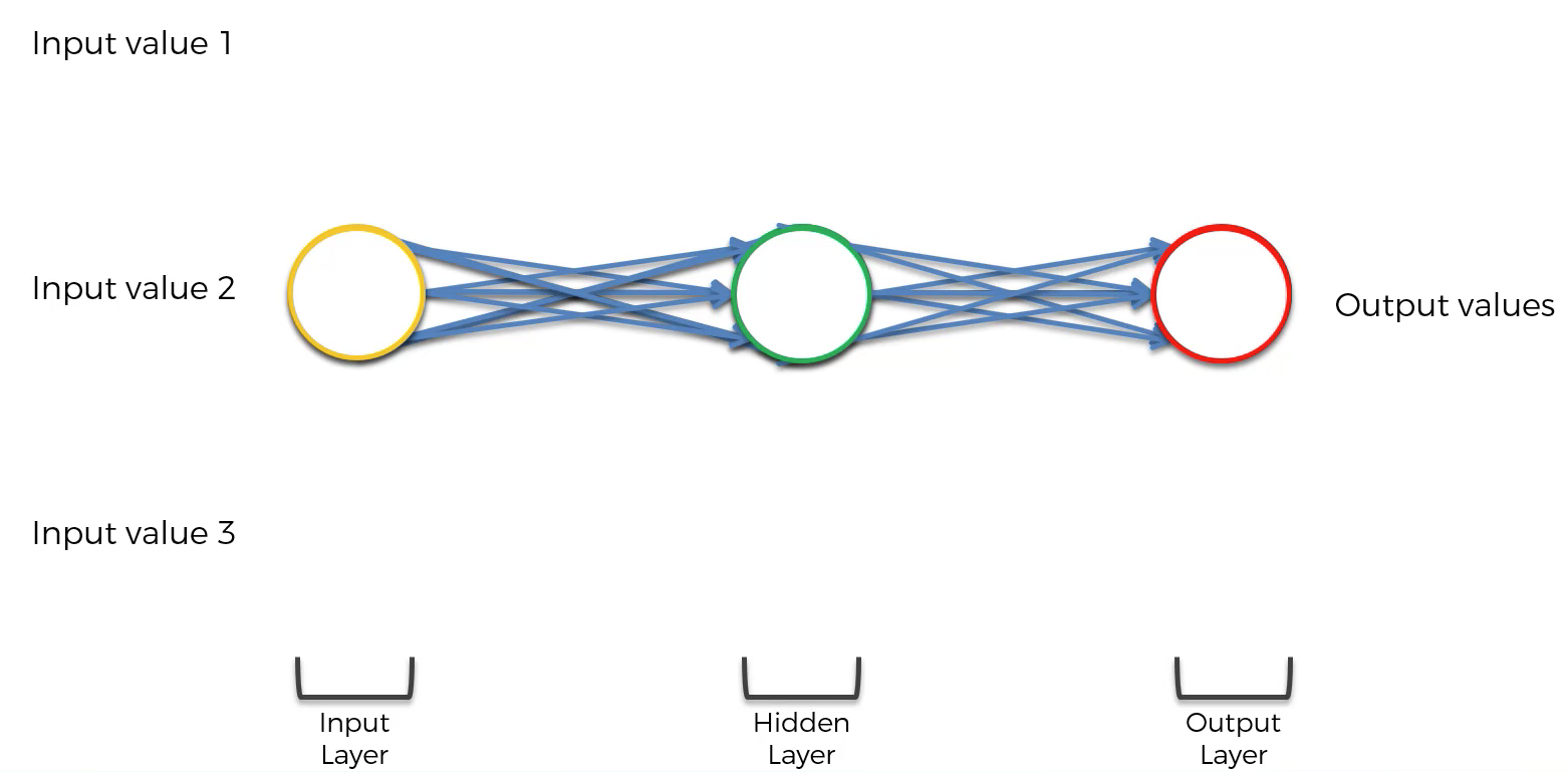
Then, three more modifications need to be made:
- The neural network’s neuron synapses need to be simplified to a single line
- The entire neural network needs to be rotated 90 degrees
- A loop needs to be generated around the hidden layer of the neural net
The neural network will now have the following appearance:
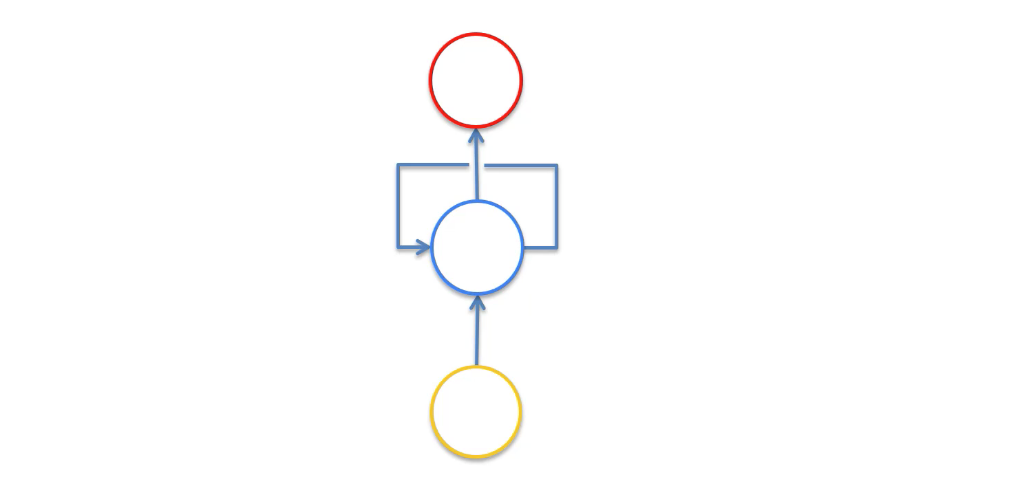
That line that circles the hidden layer of the recurrent neural network is called the temporal loop. It is used to indicate that the hidden layer not only generates an output, but that output is fed back as the input into the same layer.
A visualization is helpful in understanding this. As you can see in the following image, the hidden layer used on a specific observation of a data set is not only used to generate an output for that observation, but it is also used to train the hidden layer of the next observation.
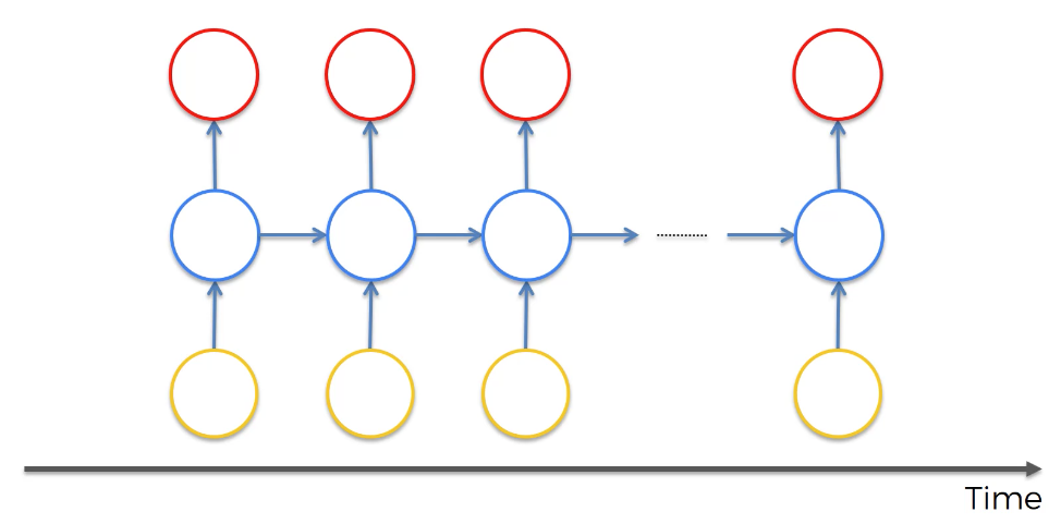
This property of one observation helping to train the next observation is why recurrent neural networks are so useful in solving time series analysis problems.
Summary – The Intuition of Recurrent Neural Networks
In this tutorial, you had your first introduction to recurrent neural networks. More specifically, we discussed the intuition behind recurrent neural networks.
Here is a brief summary of what we discussed in this tutorial:
- The types of problems solved by recurrent neural networks
- The relationships between the different parts of the brain and the different neural networks we’ve studied in this course
- The composition of a recurrent neural network and how each hidden layer can be used to help train the hidden layer from the next observation in the data set
The Vanishing Gradient Problem in Recurrent Neural Networks
The vanishing gradient problem has historically been one of the largest barriers to the success of recurrent neural networks.
Because of this, having an understanding of the vanishing gradient problem is important before you build your first RNN.
This section will explain the vanishing gradient problem in plain English, including a discussion of the most useful solutions to this interesting problem.
What Is The Vanishing Gradient Problem?
Before we dig in to the details of the vanishing gradient problem, it’s helpful to have some understanding of how the problem was initially discovered.
The vanishing gradient problem was discovered by Sepp Hochreiter, a German computer scientist who has had an influential role in the development of recurrent neural networks in deep learning.
Now let’s explore the vanishing gradient problem in detail. As its name implies, the vanishing gradient problem is related to deep learning gradient descent algorithms. Recall that a gradient descent algorithm looks something like this:
This gradient descent algorithm is then combined with a backpropagation algorithm to update the synapse weights throughout the neural network.
Recurrent neural networks behave slightly differently because the hidden layer of one observation is used to train the hidden layer of the next observation.
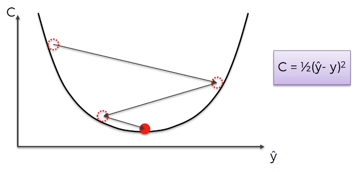
This means that the cost function of the neural net is calculated for each observation in the data set. These cost function values are depicted at the top of the following image:
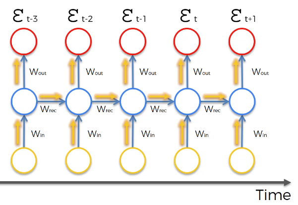
The vanishing gradient problem occurs when the backpropagation algorithm moves back through all of the neurons of the neural net to update their weights. The nature of recurrent neural networks means that the cost function computed at a deep layer of the neural net will be used to change the weights of neurons at shallower layers.
The mathematics that computes this change is multiplicative, which means that the gradient calculated in a step that is deep in the neural network will be multiplied back through the weights earlier in the network. Said differently, the gradient calculated deep in the network is “diluted” as it moves back through the net, which can cause the gradient to vanish – giving the name to the vanishing gradient problem!
The actual factor that is multiplied through a recurrent neural network in the backpropagation algorithm is referred to by the mathematical variable Wrec. It poses two problems:
- When
Wrecis small, you experience a vanishing gradient problem - When
Wrecis large, you experience an exploding gradient problem
Note that both of these problems are generally referred to by the simpler name of the “vanishing gradient problem”.
To summarize, the vanishing gradient problem is caused by the multiplicative nature of the backpropagation algorithm. It means that gradients calculated at a deep stage of the recurrent neural network either have too small of an impact (in a vanishing gradient problem) or too large of an impact (in an exploding gradient problem) on the weights of neurons that are shallower in the neural net.
How to Solve The Vanishing Gradient Problem
There are a number of strategies that can be used to solve the vanishing gradient problem. We will explore strategies for both the vanishing gradient and exploding gradient problems separately. Let’s start with the latter.
Solving the Exploding Gradient Problem
For exploding gradients, it is possible to use a modified version of the backpropagation algorithm called truncated backpropagation. The truncated backpropagation algorithm limits that number of timesteps that the backproporation will be performed on, stopping the algorithm before the exploding gradient problem occurs.
You can also introduce penalties, which are hard-coded techniques for reduces a backpropagation’s impact as it moves through shallower layers in a neural network.
Lastly, you could introduce gradient clipping, which introduces an artificial ceiling that limits how large the gradient can become in a backpropagation algorithm.
Solving the Vanishing Gradient Problem
Weight initialization is one technique that can be used to solve the vanishing gradient problem. It involves artificially creating an initial value for weights in a neural network to prevent the backpropagation algorithm from assigning weights that are unrealistically small.
You could also use echo state networks, which is a specific type of neural network designed to avoid the vanishing gradient problem. Echo state networks are outside the scope of this course. Having knowledge of their existence is sufficient for now.
The most important solution to the vanishing gradient problem is a specific type of neural network called Long Short-Term Memory Networks (LSTMs), which were pioneered by Sepp Hochreiter and Jürgen Schmidhuber. Recall that Mr. Hochreiter was the scientist who originally discovered the vanishing gradient problem.
LSTMs are used in problems primarily related to speech recognition, with one of the most notable examples being Google using an LSTM for speech recognition in 2015 and experiencing a 49% decrease in transcription errors.
LSTMs are considered to be the go-to neural net for scientists interested in implementing recurrent neural networks. We will be largely focusing on LSTMs through the remainder of this course.
Summary – The Vanishing Gradient Problem
In this section, you learned about the vanishing gradient problem of recurrent neural networks.
Here is a brief summary of what we discussed:
- That Sepp Hochreiter was the first scientist to discover the vanishing gradient problem in recurrent neural networks
- What the vanishing gradient problem (and its cousin, the exploding gradient problem) involves
- The role of
Wrecin vanishing gradient problems and exploding gradient problems - How vanishing gradient problems and exploding gradient problems are solved
- The role of LSTMs as the most common solution to the vanishing gradient problem
Long Short-Term Memory Networks (LSTMs)
Long short-term memory networks (LSTMs) are a type of recurrent neural network used to solve the vanishing gradient problem.
They differ from “regular” recurrent neural networks in important ways.
This tutorial will introduce you to LSTMs. Later in this course, we will build and train an LSTM from scratch.
Table of Contents
You can skip to a specific section of this LSTM tutorial using the table of contents below:
- The History of LSTMs
- How LSTMs Solve The Vanishing Gradient Problem
- How LSTMs Work
- Variations of LSTM Architectures
- The Peephole Variation
- The Coupled Gate Variation
- Other LSTM Variations
- Final Thoughts
The History of LSTMs
As we alluded to in the last section, the two most important figures in the field of LSTMs are Sepp Hochreiter and Jürgen Schmidhuber.
The latter was the former’s PhD supervisor at the Technical University of Munich in Germany.
Hochreiter’s PhD thesis introduced LSTMs to the world for the first time.
How LSTMs Solve The Vanishing Gradient Problem
In the last tutorial, we learned how the Wrec term in the backpropagation algorithm can lead to either a vanishing gradient problem or an exploding gradient problem.
We explored various possible solutions for this problem, including penalties, gradient clipping, and even echo state networks. LSTMs are the best solution.
So how do LSTMs work? They simply change the value of Wrec.
In our explanation of the vanishing gradient problem, you learned that:
- When
Wrecis small, you experience a vanishing gradient problem - When
Wrecis large, you experience an exploding gradient problem
We can actually be much more specific:
- When
Wrec < 1, you experience a vanishing gradient problem - When
Wrec > 1, you experience an exploding gradient problem
This makes sense if you think about the multiplicative nature of the backpropagation algorithm.
If you have a number that is smaller than 1 and you multiply it against itself over and over again, you’ll end up with a number that vanishes. Similarly, multiplying a number greater than 1 against itself many times results in a very large number.
To solve this problem, LSTMs set Wrec = 1. There is certainly more to LSTMS than setting Wrec = 1, but this is definitely the most important change that this specification of recurrent neural networks makes.
How LSTMs Work
This section will explain how LSTMs work. Before proceeding ,it’s worth mentioning that I will be using images from Christopher Olah’s blog post Understanding LSTMs, which was published in August 2015 and has some of the best LSTM visualizations that I have ever seen.
To start, let’s consider the basic version of a recurrent neural network:
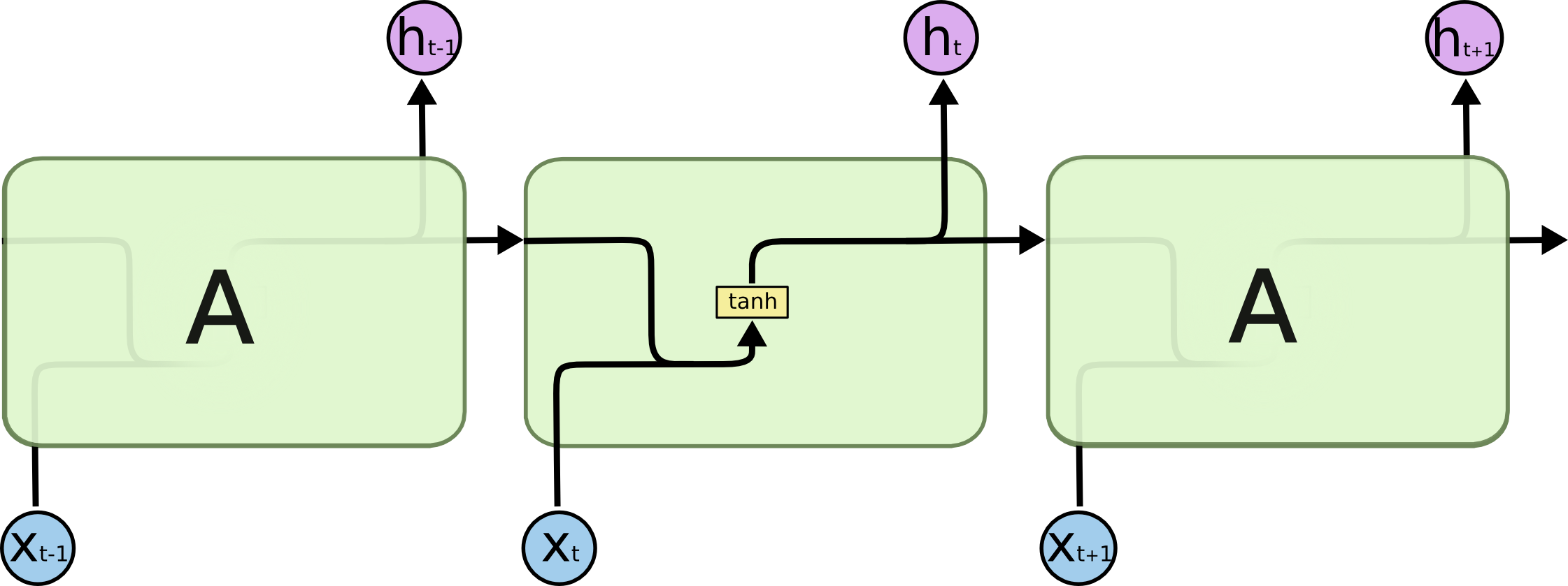
This neural network has neurons and synapses that transmit the weighted sums of the outputs from one layer as the inputs of the next layer. A backpropagation algorithm will move backwards through this algorithm and update the weights of each neuron in response to he cost function computed at each epoch of its training stage.
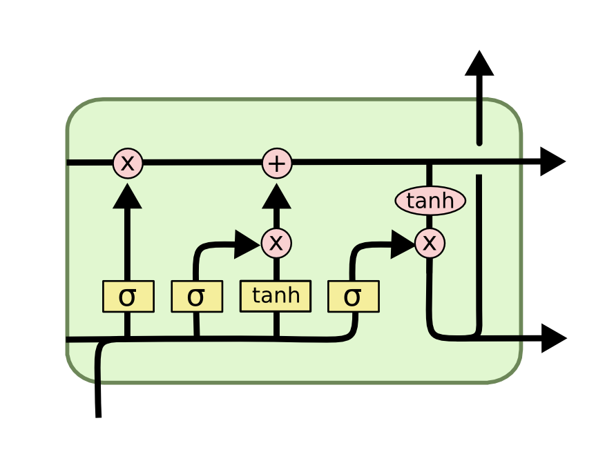
By contrast, here is what an LSTM looks like:
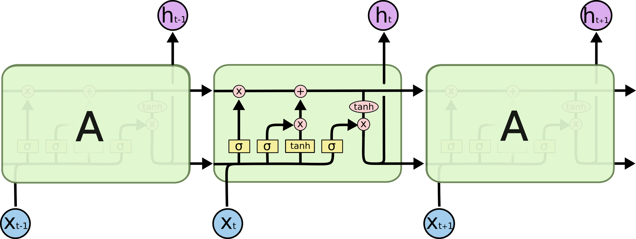
As you can see, an LSTM has far more embedded complexity than a regular recurrent neural network. My goal is to allow you to fully understand this image by the time you’ve finished this tutorial.
First, let’s get comfortable with the notation used in the image above:
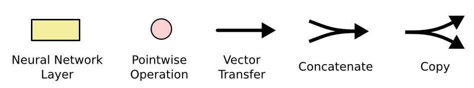
Now that you have a sense of the notation we’ll be using in this LSTM tutorial, we can start examining the functionality of a layer within an LSTM neural net. Each layer has the following appearance:
Before we dig into the functionality of nodes within an LSTM neural network, it’s worth noting that every input and output of these deep learning models is a vector. In Python, this is generally represented by a NumPy array or another one-dimensional data structure.
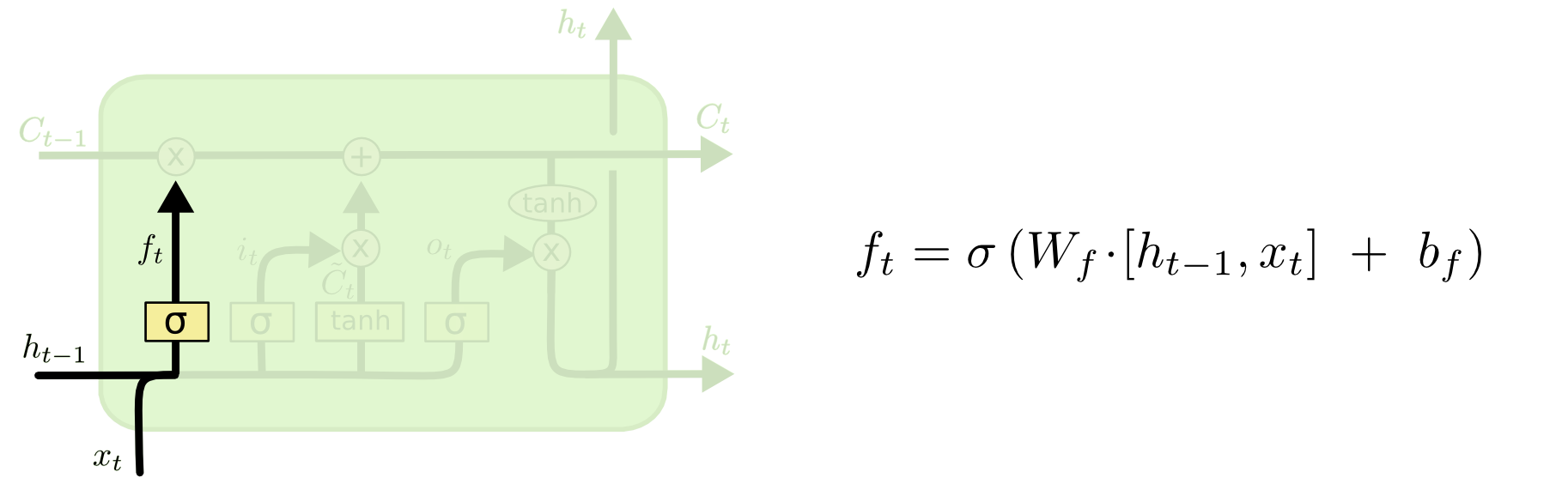
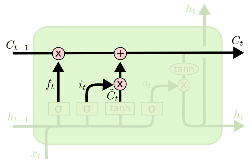
The first thing that happens within an LSTM is the activation function of the forget gate layer. It looks at the inputs of the layer (labelled xt for the observation and ht for the output of the previous layer of the neural network) and outputs either 1 or 0 for every number in the cell state from the previous layer (labelled Ct-1).
Here’s a visualization of the activation of the forget gate layer:
We have not discussed cell state yet, so let’s do that now. Cell state is represented in our diagram by the long horizontal line that runs through the top of the diagram. As an example, here is the cell state in our visualizations:
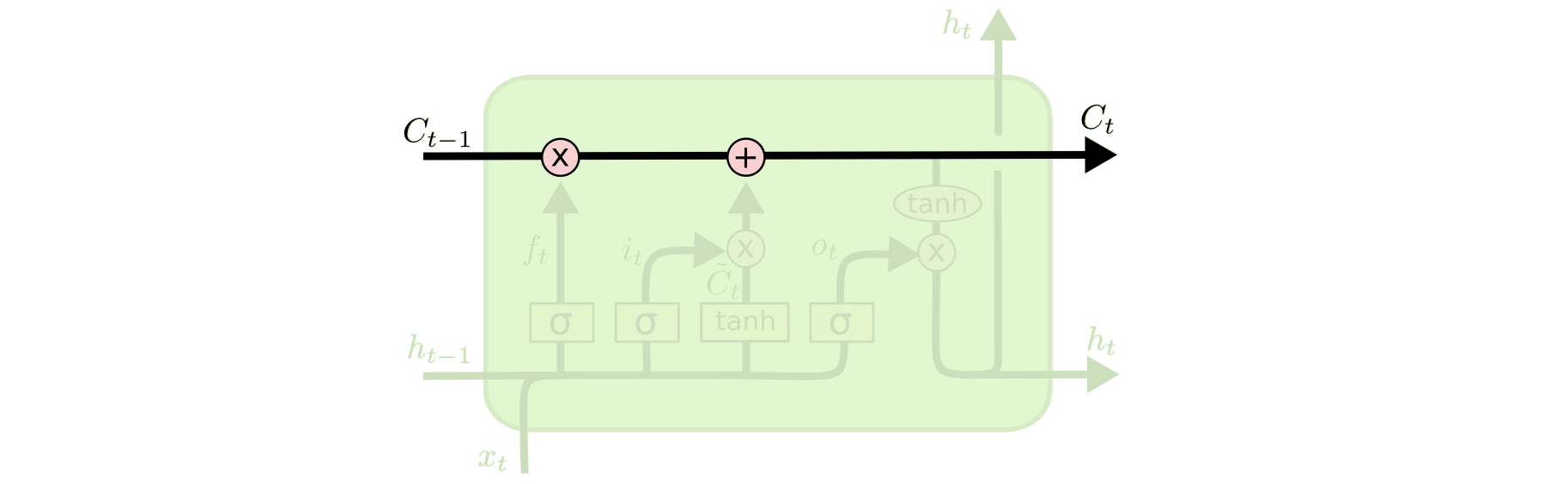
The cell state’s purpose is to decide what information to carry forward from the different observations that a recurrent neural network is trained on. The decision of whether or not to carry information forward is made by gates — of which the forget gate is a prime example. Each gate within an LSTM will have the following appearance:
The σ character within these gates refers to the Sigmoid function, which you have probably seen used in logistic regression machine learning models. The sigmoid function is used as a type of activation function in LSTMs that determines what information is passed through a gate to affect the network’s cell state.
By definition, the Sigmoid function can only output numbers between 0 and 1. It’s often used to calculate probabilities because of this. In the case of LSTM models, it specifies what proportion of each output should be allowed to influence the sell state.
The next two steps of an LSTM model are closely related: the input gate layer and the tanh layer. These layers work together to determine how to update the cell state. At the same time, the last step is completed, which allows the cell to determine what to forget about the last observation in the data set.
Here is a visualization of this process:
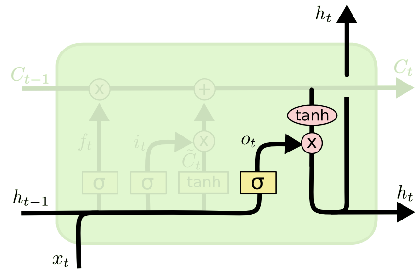
The last step of an LSTM determines the output for this observation (denoted ht). This step runs through both a sigmoid function and a hyperbolic tangent function. It can be visualized as follows:
That concludes the process of training a single layer of an LSTM model. As you might imagine, there is plenty of mathematics under the surface that we have glossed over. The point of this section is to broadly explain how LSTMs work, not for you to deeply understand each operation in the process.
Variations of LSTM Architectures
I wanted to conclude this tutorial by discussing a few different variations of LSTM architecture that are slightly different from the basic LSTM that we’ve discussed so far.
As a quick recap, here is what a generalized node of an LSTM looks like:
The Peephole Variation
Perhaps the most important variation of the LSTM architecture is the peephole variant, which allows the gate layers to read data from the cell state.
Here is a visualization of what the peephole variant might look like:
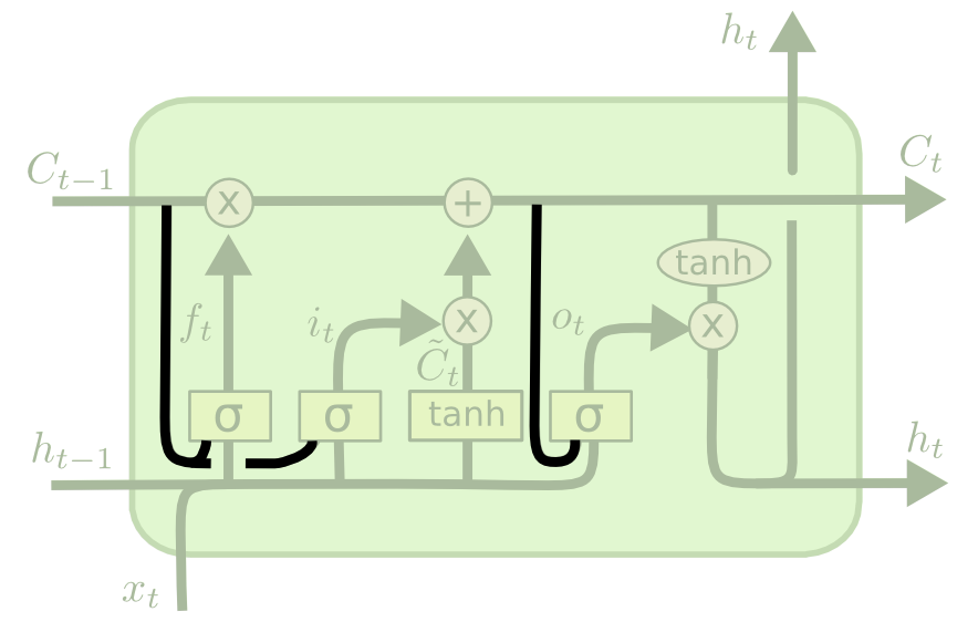
Note that while this diagram adds a peephole to every gate in the recurrent neural network, you could also add peepholes to some gates and not other gates.
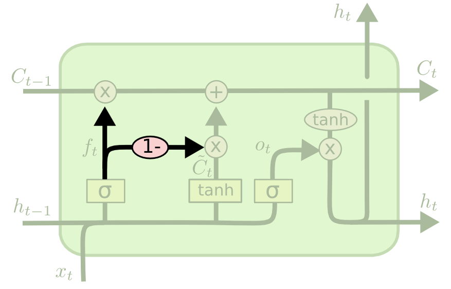
The Coupled Gate Variation
There is another variation of the LSTM architecture where the model makes the decision of what to forget and what to add new information to together. In the original LSTM model, these decisions were made separately.
Here is a visualization of what this architecture looks like:
Other LSTM Variations
These are only two examples of variants to the LSTM architecture. There are many more. A few are listed below:
- Gated Recurrent Units (GRUs)
- Depth Gated RNNs
- Clockwork RNNs
Summary — Long Short-Term Memory Networks
In this tutorial, you had your first exposure to long short-term memory networks (LSTMs).
Here is a brief summary of what you learned:
- A (very) brief history of LSTMs and the role that Sepp Hochreiter and Jürgen Schmidhuber played in their development
- How LSTMs solve the vanishing gradient problem
- How LSTMs work
- The role of gates, sigmoid functions, and the hyperbolic tangent function in LSTMs
- A few of the most popular variations of the LSTM architecture
How To Build And Train A Recurrent Neural Network
So far in our discussion of recurrent neural networks, you have learned:
- The basic intuition behind recurrent neural networks
- The vanishing gradient problem that historically impeded the progress of recurrent neural networks
- How long short-term memory networks (LSTMs) help to solve the vanishing gradient problem
It’s now time to build your first recurrent neural network! More specifically, this tutorial will teach you how to build and train an LSTM to predict the stock price of Facebook (FB).
Table of Contents
You can skip to a specific section of this Python recurrent neural network tutorial using the table of contents below:
- Downloading the Data Set For This Tutorial
- Importing The Libraries You’ll Need For This Tutorial
- Importing Our Training Set Into The Python Script
- Applying Feature Scaling To Our Data Set
- Specifying The Number Of Timesteps For Our Recurrent Neural Network
- Finalizing Our Data Sets By Transforming Them Into NumPy Arrays
- Importing Our TensorFlow Libraries
- Building Our Recurrent Neural Network
- Adding Our First LSTM Layer
- Adding Some Dropout Regularization
- Adding Three More LSTM Layers With Dropout Regularization
- Adding The Output Layer To Our Recurrent Neural Network
- Compiling Our Recurrent Neural Network
- Fitting The Recurrent Neural Network On The Training Set
- Making Predictions With Our Recurrent Neural Network
- Importing Our Test Data
- Building The Test Data Set We Need To Make Predictions
- Scaling Our Test Data
- Grouping Our Test Data
- Actually Making Predictions
- The Full Code For This Tutorial
- Final Thoughts
Downloading the Data Set For This Tutorial
To proceed through this tutorial, you will need two download two data sets:
- A set of training data that contains information on Facebook’s stock price from teh start of 2015 to the end of 2019
- A set of test data that contains information on Facebook’s stock price during the first month of 2020
Our recurrent neural network will be trained on the 2015-2019 data and will be used to predict the data from January 2020.
You can download the training data and test data using the links below:
- Training Data
- Test Data
Each of these data sets are simply exports from Yahoo! Finance. They look like this (when opened in Microsoft Excel):

Once the files are downloaded, move them to the directory you’d like to work in and open a Jupyter Notebook.
Importing The Libraries You’ll Need For This Tutorial
This tutorial will depend on a number of open-source Python libraries, including NumPy, pandas, and matplotlib.
Let’s start our Python script by importing some of these libraries:
import numpy as np

import pandas as pd

import matplotlib.pyplot as plt
Importing Our Training Set Into The Python Script
The next task that needs to be completed is to import our data set into the Python script.
We will initially import the data set as a pandas DataFrame using the read_csv method. However, since the keras module of TensorFlow only accepts NumPy arrays as parameters, the data structure will need to be transformed post-import.
Let’s start by importing the entire .csv file as a DataFrame:
training_data = pd.read_csv('FB_training_data.csv')
You will notice in looking at the DataFrame that it contains numerous different ways of measuring Facebook’s stock price, including opening price, closing price, high and low prices, and volume information:
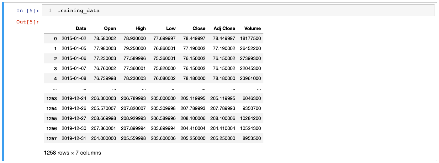
We will need to select a specific type of stock price before proceeding. Let’s use Close, which indicates the unadjusted closing price of Facebook’s stock.
Now we need to select that column of the DataFrame and store it in a NumPy array. Here is the command to do this:
training_data = training_data.iloc[:, 1].values
Note that this command overwrites the existing training_data variable that we had created previously.
You can now verify that our training_data variable is indeed a NumPy array by running type(training_data), which should return:
numpy.ndarray
Applying Feature Scaling To Our Data Set
Let’s now take some time to apply some feature scaling to our data set.
As a quick refresher, there are two main ways that you can apply featuer scaling to your data set:
- Standardization
- Normalization
We’ll be using normalization to build our recurrent neural network, which involves subtracting the minimum value of the data set and then dividing by the range of the data set.
Here is the normalization function defined mathematically:
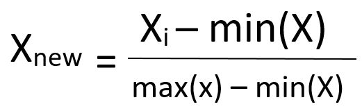
Fortunately, scikit-learn makes it very easy to apply normalization to a dataset using its MinMaxScaler class.
Let’s start by importing this class into our Python script. The MinMaxScaler class lives within the preprocessing module of scikit-learn, so the command to import the class is:
from sklearn.preprocessing import MinMaxScaler
Next we need to create an instance of this class. We will assign the newly-created object to a variable called scaler. We will be using the default parameters for this class, so we do not need to pass anything in:
scaler = MinMaxScaler()
Since we haven’t specified any non-default parameters, this will scale our data set so that every observation is between 0 and 1.
We have created our scaler object but our training_data data set has not yet been scaled. We need to use the fit_transform method to modify the original data set. Here’s the statement to do this:
training_data = scaler.fit_transform(training_data.reshape(-1, 1))
Specifying The Number Of Timesteps For Our Recurrent Neural Network
The next thing we need to do is to specify our number of timesteps. Timesteps specify how many previous observations should be considered when the recurrent neural network makes a prediction about the current observation.
We will use 40 timesteps in this tutorial. This means that for every day that the neural network predicts, it will consider the previous 40 days of stock prices to determine its output. Note that since there are only ~20 trading days in a given month, using 40 timesteps means we’re relying on stock price data from the previous 2 months.
So how do we actually specify the number of timesteps within our Python script?
It’s done through creating two special data structures:
- One data structure that we’ll call
x_training_datathat contains the last 40 stock price observations in the data set. This is the data that the recurrent neural network will use to make predictions. - One data structure that we’ll call
y_training_datathat contains the stock price for the next trading day. This is the data point that the recurrent neural network is trying to predict.
To start, let’s initialize each of these data structures as an empty Python list:
x_training_data = []

y_training_data =[]
Now we will use a for loop to populate the actual data into each of these Python lists. Here’s the code (with further explanation of the code after the code block):
for i in range(40, len(training_data)):

    x_training_data.append(training_data[i-40:i, 0])

    y_training_data.append(training_data[i, 0])
Let’s unpack the components of this code block:
- The
range(40, len(training_data))function causes the for loop to iterate from40to the last index of the training data. - The
x_training_data.append(training_data[i-40:i, 0])line causes the loop to append the 40 preceding stock prices tox_training_datawith each iteration of the loop. - Similarly, the
y_training_data.append(training_data[i, 0])causes the loop to append the next day’s stock price toy_training_datawith each iteration of the loop.
Finalizing Our Data Sets By Transforming Them Into NumPy Arrays
TensorFlow is designed to work primarily with NumPy arrays. Because of this, the last thing we need to do is transform the two Python lists we just created into NumPy arrays.
Fortunately, this is simple. You simply need to wrap the Python lists in the np.array function. Here’s the code:
x_training_data = np.array(x_training_data)

y_training_data = np.array(y_training_data)
One important way that you can make sure your script is running as intended is to verify the shape of both NumPy arrays.
The x_training_data array should be a two-directional NumPy array with one dimension being 40 (the number of timesteps) and the second dimension being len(training_data) - 40, which evaluates to 1218 in our case.
Similarly, the y_training_data object should be a one-dimensional NumPy array of length 1218 (which, again, is len(training_data) - 40).
You can verify the shape of the arrays by printing their shape attribute, like this:
print(x_training_data.shape)

print(y_training_data.shape)
This prints:
(1218, 40)

(1218,)
Both arrays have the dimensions you’d expect. However, we need to reshape our x_training_data object one more time before proceeding to build our recurrent neural network.
The reason for this is that the recurrent neural network layer available in TensorFlow only accepts data in a very specific format. You can read the TensorFlow documentation on this topic here.
To reshape the x_training_data object, I will use the np.reshape method. Here’s the code to do this:
x_training_data = np.reshape(x_training_data, (x_training_data.shape[0],

                                               x_training_data.shape[1],

                                               1))
Now let’s print the shape of x_training_data once again:
print(x_training_data.shape)
This outputs:
(1218, 40, 1)
Our arrays have the desired shape, so we can proceed to building our recurrent neural network.
Importing Our TensorFlow Libraries
Before we can begin building our recurrent neural network, we’ll need to import a number of classes from TensorFlow. Here are the statements you should run before proceeding:
from tensorflow.keras.models import Sequential

from tensorflow.keras.layers import Dense

from tensorflow.keras.layers import LSTM

from tensorflow.keras.layers import Dropout
Building Our Recurrent Neural Network
It’s now time to build our recurrent neural network.
The first thing that needs to be done is initializing an object from TensorFlow’s Sequential class. As its name implies, the Sequential class is designed to build neural networks by adding sequences of layers over time.
Here’s the code to initialize our recurrent neural network:
rnn = Sequential()
As with our artificial neural networks and convolutional neural networks, we can add more layers to this recurrent neural network using the add method.
Adding Our First LSTM Layer
The first layer that we will add is an LSTM layer. To do this, pass an invocation of the LSTM class (that we just imported) into the add method.
The LSTM class accepts several parameters. More precisely, we will specify three arguments:
- The number of LSTM neurons that you’d like to include in this layer. Increasing the number of neurons is one method for increasing the dimensionality of your recurrent neural network. In our case, we will specify
units = 45. return_sequences = True— this must always be specified if you plan on including another LSTM layer after the one you’re adding. You should specifyreturn_sequences = Falsefor the last LSTM layer in your recurrent neural network.input_shape: the number of timesteps and the number of predictors in our training data. In our case, we are using40timesteps and only1predictor (stock price), so we will add
Here is the full add method:
rnn.add(LSTM(units = 45, return_sequences = True, input_shape = (x_training_data.shape[1], 1)))
Note that I used x_training_data.shape[1] instead of the hardcoded value in case we decide to train the recurrent neural network on a larger model at a later date.
Adding Some Dropout Regularization
Dropout regularization is a technique used to avoid overfitting when training neural networks.
It involves randomly excluding — or “dropping out” — certain layer outputs during the training stage.
TensorFlow makes it easy to implement dropout regularization using the Dropout class that we imported earlier in our Python script. The Dropout class accepts a single parameter: the dropout rate.
The dropout rate indicates how many neurons should be dropped in a specific layer of the neural network. It is common to use a dropout rate of 20%. We will follow this convention in our recurrent neural network.
Here’s how you can instruct TensorFlow to drop 20% of the LSTM layer’s neuron during each iteration of the training stage:
rnn.add(Dropout(0.2))
Adding Three More LSTM Layers With Dropout Regularization
We will now add three more LSTM layers (with dropout regularization) to our recurrent neural network. You will see that after specifying the first LSTM layer, adding more is trivial.
To add more layers, all that needs to be done is copying the first two add methods with one small change. Namely, we should remove the input_shape argument from the LSTM class.
We will keep the number of neurons (or units) and the dropout rate the same in each of the LSTM class invocations. Since the third LSTM layer we’re adding in this section will be our last LSTM layer, we can remove the return_sequences = True parameter as mentioned earlier. Removing the parameter sets return_sequences to its default value of False.
Here’s the full code to add our next three LSTM layers:
rnn.add(LSTM(units = 45, return_sequences = True))

rnn.add(Dropout(0.2))

rnn.add(LSTM(units = 45, return_sequences = True))

rnn.add(Dropout(0.2))

rnn.add(LSTM(units = 45))

rnn.add(Dropout(0.2))
This code is very repetitive and violates the DRY (Don’t repeat yourself) principle of software development. Let’s nest it in a loop instead:
for i in [True, True, False]:

    rnn.add(LSTM(units = 45, return_sequences = i))

    rnn.add(Dropout(0.2))
Adding The Output Layer To Our Recurrent Neural Network
Let’s finish architecting our recurrent neural network by adding our output layer.
The output layer will be an instance of the Dense class, which is the same class we used to create the full connection layer of our convolutional neural network earlier in this course.
The only parameter we need to specify is units , which is the desired number of dimensions that the output layer should generate. Since we want to output the next day’s stock price (a single value), we’ll specify units = 1.
Here’s the code to create our output layer:
rnn.add(Dense(units = 1))
Compiling Our Recurrent Neural Network
As you’ll recall from the tutorials on artificial neural networks and convolutional neural networks, the compilation step of building a neural network is where we specify the neural net’s optimizer and loss function.
TensorFlow allows us to compile a neural network using the aptly-named compile method. It accepts two arguments: optimizer and loss. Let’s start by creating an empty compile function:
rnn.compile(optimizer = '', loss = '')
We now need to specify the optimizer and loss parameters.
Let’s start by discussing the optimizer parameter. Recurrent neural networks typically use the RMSProp optimizer in their compilation stage. With that said, we will use the Adam optimizer (as before). The Adam optimizer is a workhorse optimizer that is useful in a wide variety of neural network architectures.
The loss parameter is fairly simple. Since we’re predicting a continuous variable, we can use mean squared error — just like you would when measuring the performance of a linear regression machine learning model. This means we can specify loss = mean_squared_error.
Here’s the final compile method:
rnn.compile(optimizer = 'adam', loss = 'mean_squared_error')
Fitting The Recurrent Neural Network On The Training Set
It’s now time to train our recurrent network on our training data.
To do this, we use the fit method. The fit method accepts four arguments in this case:
- The training data: in our case, this will be
x_training_dataandy_training_data - Epochs: the number of iterations you’d like the recurrent neural network to be trained on. We will specify
epochs = 100in this case. - The batch size: the size of batches that the network will be trained in through each epoch.
Here is the code to train this recurrent neural network according to our specifications:
rnn.fit(x_training_data, y_training_data, epochs = 100, batch_size = 32)
Your Jupyter Notebook will now generate a number of printed outputs for every epoch in the training algorithm. They look like this:
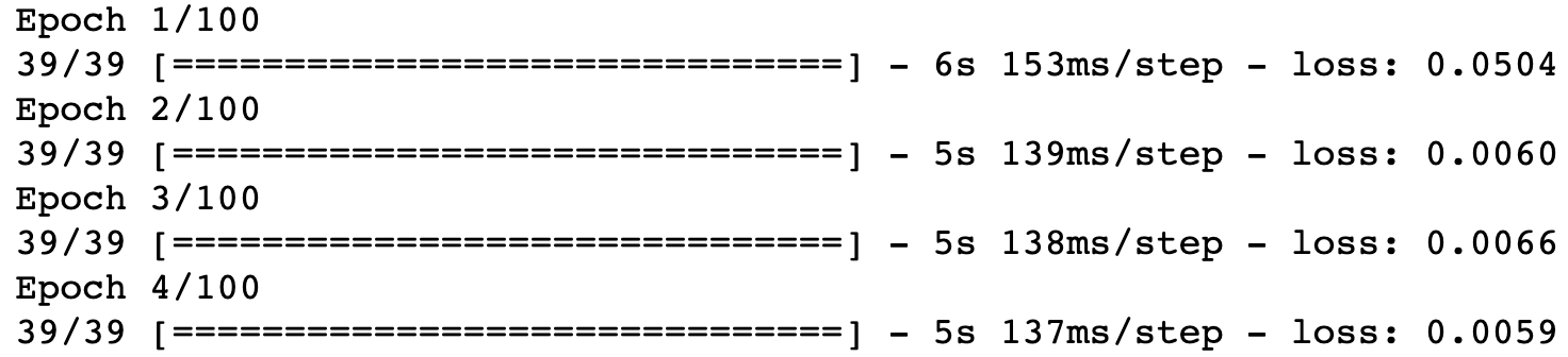
As you can see, every output shows how long the epoch took to compute as well as the computed loss function at that epoch.
You should see the loss function’s value slowly decline as the recurrent neural network is fitted to the training data over time. In my case, the loss function’s value declined from 0.0504 in the first iteration to 0.0017 in the last iteration.
Making Predictions With Our Recurrent Neural Network
We have built our recurrent neural network and trained it on data of Facebook’s stock price over the last 5 years. It’s now time to make some predictions!
Importing Our Test Data
To start, let’s import the actual stock price data for the first month of 2020. This will give us something to compare our predicted values to.
Here’s the code to do this. Note that it is very similar to the code that we used to import our training data at the start of our Python script:
test_data = pd.read_csv('FB_test_data.csv')

test_data = test_data.iloc[:, 1].values
If you run the statement print(test_data.shape), it will return (21,). This shows that our test data is a one-dimensional NumPy array with 21 entries — which means there were 21 stock market trading days in January 2020.
You can also generate a quick plot of the data using plt.plot(test_data). This should generate the following Python visualization:
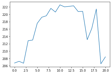
With any luck, our predicted values should follow the same distribution.
Building The Test Data Set We Need To Make Predictions
Before we can actually make predictions for Facebook’s stock price in January 2020, we first need to make some changes to our data set.
The reason for this is that to predict each of the 21 observations in January, we will need the 40 previous trading days. Some of these trading days will come from the test set while the remainder will come from the training set. Because of this, some concatenation is necessary.
Unfortunately, you can just concatenate the NumPy arrays immediately. This is because we’ve already applied feature scaling to the training data but haven’t applied any feature scaling to the test data.
To fix this, we need to re-import the original x_training_data object under a new variable name called unscaled_x_training_data. For consistency, we will also re-import the test data as a DataFrame called unscaled_test_data:
unscaled_training_data = pd.read_csv('FB_training_data.csv')

unscaled_test_data = pd.read_csv('FB_test_data.csv')
Now we can concatenate together the Open column from each DataFrame with the following statement:
all_data = pd.concat((unscaled_x_training_data['Open'], unscaled_test_data['Open']), axis = 0)
This all_data object is a pandas Series of length 1279.
Now we need to create an array of all the stock prices from January 2020 and the 40 trading days prior to January. We will call this object x_test_data since it contains the x values that we’ll use to make stock price predictions for January 2020.
The first thing you need to do is find the index of the first trading day in January within our all_data object. The statement len(all_data) - len(test_data) identifies this index for us.
This represents the upper bound of the first item in the array. To get the lower bound, just subtract 40 from this number. Said differently, the lower bound is len(all_data) - len(test_data) - 40.
The upper bound of the entire x_test_data array will be the last item in the data set. Accordingly, we can create this NumPy array with the following statement:
x_test_data = all_data[len(all_data) - len(test_data) - 40:].values
You can check whether or not this object has been created as desired by printing len(x_test_data), which has a value of 61. This makes sense — it should contain the 21 values for January 2020 as well as the 40 values prior.
The last step of this section is to quickly reshape our NumPy array to make it suitable for the predict method:
x_test_data = np.reshape(x_test_data, (-1, 1))
Note that if you neglected to do this step, TensorFlow would print a handy message that would explain exactly how you’d need to transform your data.
Scaling Our Test Data
Our recurrent neural network was trained on scaled data. Because of this, we need to scale our x_test_data variable before we can use the model to make predictions.
x_test_data = scaler.transform(x_test_data)
Note that we used the transform method here instead of the fit_transform method (like before). This is because we want to transform the test data according to the fit generated from the entire training data set.
This means that the transformation that is applied to the test data will be the same as the one applied to the training data — which is necessary for our recurrent neural network to make accurate predictions.
Grouping Our Test Data
The last thing we need to do is group our test data into 21 arrays of size 40. Said differently, we’ll now create an array where each entry corresponds to a date in January and contains the stock prices of the 40 previous trading days.
The code to do this is similar to something we used earlier:
final_x_test_data = []

for i in range(40, len(x_test_data)):

    final_x_test_data.append(x_test_data[i-40:i, 0])

final_x_test_data = np.array(final_x_test_data)
Lastly, we need to reshape the final_x_test_data variable to meet TensorFlow standards.
We saw this previously, so the code should need no explanation:
final_x_test_data = np.reshape(final_x_test_data, (final_x_test_data.shape[0],

                                               final_x_test_data.shape[1],

                                               1))
Actually Making Predictions
After an absurd amount of data reprocessing, we are now ready to make predictions using our test data!
This step is simple. Simply pass in our final_x_test_data object into the predict method called on the rnn object. As an example, here is how you could generate these predictions and store them in an aptly-named variable called predictions:
predictions = rnn.predict(final_x_test_data)
Let’s plot these predictions by running plt.plot(predictions) (note that you’ll need to run plt.clf() to clear your canvas first):
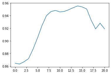
As you can see, the predicted values in this plot are all between 0 and 1. This is because our data set is still scaled! We need to un-scale it for the predictions to have any practical meaning.
The MinMaxScaler class that we used to originally scale our data set comes with a useful inverse_transform method to un-scale the data. Here’s how you could un-scale the data and generate a new plot:
unscaled_predictions = scaler.inverse_transform(predictions)

plt.clf() #This clears the first prediction plot from our canvas

plt.plot(unscaled_predictions)
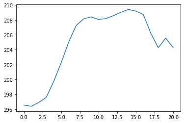
This looks much better! Anyone who’s followed Facebook’s stock price for any length of time can see that this seems fairly close to where Facebook has actually traded.
Let’s generate plot that compares our predicted stock prices with Facebook’s actual stock price:
plt.plot(unscaled_predictions, color = '#135485', label = "Predictions")

plt.plot(test_data, color = 'black', label = "Real Data")

plt.title('Facebook Stock Price Predictions')
The Full Code For This Tutorial
You can view the full code for this tutorial in this GitHub repository. It is also pasted below for your reference:
#Import the necessary data science libraries

import numpy as np

import pandas as pd

import matplotlib.pyplot as plt

#Import the data set as a pandas DataFrame

training_data = pd.read_csv('FB_training_data.csv')

#Transform the data set into a NumPy array

training_data = training_data.iloc[:, 1].values

#Apply feature scaling to the data set

from sklearn.preprocessing import MinMaxScaler

scaler = MinMaxScaler()

training_data = scaler.fit_transform(training_data.reshape(-1, 1))

#Initialize our x_training_data and y_training_data variables

#as empty Python lists

x_training_data = []

y_training_data =[]

#Populate the Python lists using 40 timesteps

for i in range(40, len(training_data)):

    x_training_data.append(training_data[i-40:i, 0])

    y_training_data.append(training_data[i, 0])


#Transforming our lists into NumPy arrays

x_training_data = np.array(x_training_data)

y_training_data = np.array(y_training_data)

#Verifying the shape of the NumPy arrays

print(x_training_data.shape)

print(y_training_data.shape)

#Reshaping the NumPy array to meet TensorFlow standards

x_training_data = np.reshape(x_training_data, (x_training_data.shape[0],

                                               x_training_data.shape[1],

                                               1))

#Printing the new shape of x_training_data

print(x_training_data.shape)

#Importing our TensorFlow libraries

from tensorflow.keras.models import Sequential

from tensorflow.keras.layers import Dense

from tensorflow.keras.layers import LSTM

from tensorflow.keras.layers import Dropout

#Initializing our recurrent neural network

rnn = Sequential()

#Adding our first LSTM layer

rnn.add(LSTM(units = 45, return_sequences = True, input_shape = (x_training_data.shape[1], 1)))

#Perform some dropout regularization

rnn.add(Dropout(0.2))

#Adding three more LSTM layers with dropout regularization

for i in [True, True, False]:

    rnn.add(LSTM(units = 45, return_sequences = i))

    rnn.add(Dropout(0.2))

#(Original code for the three additional LSTM layers)

# rnn.add(LSTM(units = 45, return_sequences = True))

# rnn.add(Dropout(0.2))

# rnn.add(LSTM(units = 45, return_sequences = True))

# rnn.add(Dropout(0.2))

# rnn.add(LSTM(units = 45))

# rnn.add(Dropout(0.2))

#Adding our output layer

rnn.add(Dense(units = 1))

#Compiling the recurrent neural network

rnn.compile(optimizer = 'adam', loss = 'mean_squared_error')

#Training the recurrent neural network

rnn.fit(x_training_data, y_training_data, epochs = 100, batch_size = 32)

#Import the test data set and transform it into a NumPy array

test_data = pd.read_csv('FB_test_data.csv')

test_data = test_data.iloc[:, 1].values

#Make sure the test data's shape makes sense

print(test_data.shape)

#Plot the test data

plt.plot(test_data)

#Create unscaled training data and test data objects

unscaled_training_data = pd.read_csv('FB_training_data.csv')

unscaled_test_data = pd.read_csv('FB_test_data.csv')

#Concatenate the unscaled data

all_data = pd.concat((unscaled_x_training_data['Open'], unscaled_test_data['Open']), axis = 0)

#Create our x_test_data object, which has each January day + the 40 prior days

x_test_data = all_data[len(all_data) - len(test_data) - 40:].values

x_test_data = np.reshape(x_test_data, (-1, 1))

#Scale the test data

x_test_data = scaler.transform(x_test_data)

#Grouping our test data

final_x_test_data = []

for i in range(40, len(x_test_data)):

    final_x_test_data.append(x_test_data[i-40:i, 0])

final_x_test_data = np.array(final_x_test_data)

#Reshaping the NumPy array to meet TensorFlow standards

final_x_test_data = np.reshape(final_x_test_data, (final_x_test_data.shape[0],

                                               final_x_test_data.shape[1],

                                               1))

#Generating our predicted values

predictions = rnn.predict(final_x_test_data)

#Plotting our predicted values

plt.clf() #This clears the old plot from our canvas

plt.plot(predictions)

#Unscaling the predicted values and re-plotting the data

unscaled_predictions = scaler.inverse_transform(predictions)

plt.clf() #This clears the first prediction plot from our canvas

plt.plot(unscaled_predictions)

#Plotting the predicted values against Facebook's actual stock price

plt.plot(unscaled_predictions, color = '#135485', label = "Predictions")

plt.plot(test_data, color = 'black', label = "Real Data")

plt.title('Facebook Stock Price Predictions')
Summary — The Intuition Behind Recurrent Neural Networks
In this tutorial, you learned how to build and train a recurrent neural network.
Here is a brief summary of what you learned:
- How to apply feature scaling to a data set that a recurrent neural network will be trained on
- The role of
timestepsin training a recurrent neural network - That TensorFlow primarily uses NumPy arrays as the data structure to train models with
- How to add
LSTMandDropoutlayers to a recurrent neural network - Why dropout regularization is commonly used to avoid overfitting when training neural networks
- That the
Denselayer from TensorFlow is commonly used as the output layer of a recurrent neural network - That the
compilationstep of building a neural network involves specifying its optimizer and its loss function - How to make predictions using a recurrent neural network
- That predictions make using a neural network trained on scaled data must be unscaled to be interpretable by humans
If you found this post helpful, check out my book Pragmatic Machine Learning for a project-based guide on deep learning models covered here and in my other articles.
Pragmatic Machine Learning
Machine learning is changing the world. But it's always been hard to learn machine learning… until now.Pragmatic Machine Learning is a step-by-step guide that will teach you machine learning fundamentals through building 9 real-world projects.You'll learn:Linear regressionLogistic regressi…
![]() Nick McCullumGumroad
Nick McCullumGumroad

Learn to code for free. freeCodeCamp’s open source curriculum has helped more than 40,000 people get jobs as developers. Get started
Recurrent neural networks are deep learning models that are typically used to solve time series problems. They are used in self-driving cars, high-frequency trading algorithms, and other real-world applications.
This tutorial will teach you the fundamentals of recurrent neural networks. You’ll also build your own recurrent neural network that predicts tomorrow’s stock price for Facebook (FB).
The Intuition of Recurrent Neural Networks
Recurrent neural networks are an example of the broader field of neural networks. Other examples include:
- Artificial neural networks
- Convolutional neural networks
This article will be focused on recurrent neural networks.
This tutorial will begin our discussion of recurrent neural networks by discussing the intuition behind recurrent neural networks.
The Types of Problems Solved By Recurrent Neural Networks
Although we have not explicitly discussed it yet, there are generally broad swathes of problems that each type of neural network is designed to solve:
- Artificial neural networks: classification and regression problems
- Convolutional neural networks: computer vision problems
In the case of recurrent neural networks, they are typically used to solve time series analysis problems.
Each of these three types of neural networks (artificial, convolutional, and recurrent) are used to solve supervised machine learning problems.
Mapping Neural Networks to Parts of the Human Brain
As you’ll recall, neural networks were designed to mimic the human brain. This is true for both their construction (both the brain and neural networks are composed of neurons) and their function (they are both used to make decisions and predictions).
The three main parts of the brain are:
- The cerebrum
- The brainstem
- The cerebellum
Arguably the most important part of the brain is the cerebrum. It contains four lobes:
- The frontal lobe
- The parietal lobe
- The temporal lobe
- The occipital lobe
The main innovation that neural networks contain is the idea of weights.
Said differently, the most important characteristic of the brain that neural networks have mimicked is the ability to learn from other neurons.
The ability of a neural network to change its weights through each epoch of its training stage is similar to the long-term memory that is seen in humans (and other animals).
The temporal lobe is the part of the brain that is associated with long-term memory. Separately, the artificial neural network was the first type of neural network that had this long-term memory property. In this sense, many researchers have compared artificial neural networks with the temporal lobe of the human brain.
Similarly, the occipital lobe is the component of the brain that powers our vision. Since convolutional neural networks are typically used to solve computer vision problems, you could say that they are equivalent to the occipital lobe in the brain.
As mentioned, recurrent neural networks are used to solve time series problems. They can learn from events that have happened in recent previous iterations of their training stage. In this way, they are often compared to the frontal lobe of the brain – which powers our short-term memory.
To summarize, researchers often pair each of the three neural nets with the following parts of the brain:
- Artificial neural networks: the temporal lobe
- Convolutional neural networks: the occipital lobe
- Recurrent neural networks: the frontal lobe
The Composition of a Recurrent Neural Network
Let’s now discuss the composition of a recurrent neural network. First, recall that the composition of a basic neural network has the following appearance:
The first modification that needs to be made to this neural network is that each layer of the network should be squashed together, like this:
Then, three more modifications need to be made:
- The neural network’s neuron synapses need to be simplified to a single line
- The entire neural network needs to be rotated 90 degrees
- A loop needs to be generated around the hidden layer of the neural net
The neural network will now have the following appearance:
That line that circles the hidden layer of the recurrent neural network is called the temporal loop. It is used to indicate that the hidden layer not only generates an output, but that output is fed back as the input into the same layer.
A visualization is helpful in understanding this. As you can see in the following image, the hidden layer used on a specific observation of a data set is not only used to generate an output for that observation, but it is also used to train the hidden layer of the next observation.
This property of one observation helping to train the next observation is why recurrent neural networks are so useful in solving time series analysis problems.
Summary – The Intuition of Recurrent Neural Networks
In this tutorial, you had your first introduction to recurrent neural networks. More specifically, we discussed the intuition behind recurrent neural networks.
Here is a brief summary of what we discussed in this tutorial:
- The types of problems solved by recurrent neural networks
- The relationships between the different parts of the brain and the different neural networks we’ve studied in this course
- The composition of a recurrent neural network and how each hidden layer can be used to help train the hidden layer from the next observation in the data set
The Vanishing Gradient Problem in Recurrent Neural Networks
The vanishing gradient problem has historically been one of the largest barriers to the success of recurrent neural networks.
Because of this, having an understanding of the vanishing gradient problem is important before you build your first RNN.
This section will explain the vanishing gradient problem in plain English, including a discussion of the most useful solutions to this interesting problem.
What Is The Vanishing Gradient Problem?
Before we dig in to the details of the vanishing gradient problem, it’s helpful to have some understanding of how the problem was initially discovered.
The vanishing gradient problem was discovered by Sepp Hochreiter, a German computer scientist who has had an influential role in the development of recurrent neural networks in deep learning.
Now let’s explore the vanishing gradient problem in detail. As its name implies, the vanishing gradient problem is related to deep learning gradient descent algorithms. Recall that a gradient descent algorithm looks something like this:
This gradient descent algorithm is then combined with a backpropagation algorithm to update the synapse weights throughout the neural network.
Recurrent neural networks behave slightly differently because the hidden layer of one observation is used to train the hidden layer of the next observation.
This means that the cost function of the neural net is calculated for each observation in the data set. These cost function values are depicted at the top of the following image:
The vanishing gradient problem occurs when the backpropagation algorithm moves back through all of the neurons of the neural net to update their weights. The nature of recurrent neural networks means that the cost function computed at a deep layer of the neural net will be used to change the weights of neurons at shallower layers.
The mathematics that computes this change is multiplicative, which means that the gradient calculated in a step that is deep in the neural network will be multiplied back through the weights earlier in the network. Said differently, the gradient calculated deep in the network is “diluted” as it moves back through the net, which can cause the gradient to vanish – giving the name to the vanishing gradient problem!
The actual factor that is multiplied through a recurrent neural network in the backpropagation algorithm is referred to by the mathematical variable Wrec. It poses two problems:
- When
Wrecis small, you experience a vanishing gradient problem - When
Wrecis large, you experience an exploding gradient problem
Note that both of these problems are generally referred to by the simpler name of the “vanishing gradient problem”.
To summarize, the vanishing gradient problem is caused by the multiplicative nature of the backpropagation algorithm. It means that gradients calculated at a deep stage of the recurrent neural network either have too small of an impact (in a vanishing gradient problem) or too large of an impact (in an exploding gradient problem) on the weights of neurons that are shallower in the neural net.
How to Solve The Vanishing Gradient Problem
There are a number of strategies that can be used to solve the vanishing gradient problem. We will explore strategies for both the vanishing gradient and exploding gradient problems separately. Let’s start with the latter.
Solving the Exploding Gradient Problem
For exploding gradients, it is possible to use a modified version of the backpropagation algorithm called truncated backpropagation. The truncated backpropagation algorithm limits that number of timesteps that the backproporation will be performed on, stopping the algorithm before the exploding gradient problem occurs.
You can also introduce penalties, which are hard-coded techniques for reduces a backpropagation’s impact as it moves through shallower layers in a neural network.
Lastly, you could introduce gradient clipping, which introduces an artificial ceiling that limits how large the gradient can become in a backpropagation algorithm.
Solving the Vanishing Gradient Problem
Weight initialization is one technique that can be used to solve the vanishing gradient problem. It involves artificially creating an initial value for weights in a neural network to prevent the backpropagation algorithm from assigning weights that are unrealistically small.
You could also use echo state networks, which is a specific type of neural network designed to avoid the vanishing gradient problem. Echo state networks are outside the scope of this course. Having knowledge of their existence is sufficient for now.
The most important solution to the vanishing gradient problem is a specific type of neural network called Long Short-Term Memory Networks (LSTMs), which were pioneered by Sepp Hochreiter and Jürgen Schmidhuber. Recall that Mr. Hochreiter was the scientist who originally discovered the vanishing gradient problem.
LSTMs are used in problems primarily related to speech recognition, with one of the most notable examples being Google using an LSTM for speech recognition in 2015 and experiencing a 49% decrease in transcription errors.
LSTMs are considered to be the go-to neural net for scientists interested in implementing recurrent neural networks. We will be largely focusing on LSTMs through the remainder of this course.
Summary – The Vanishing Gradient Problem
In this section, you learned about the vanishing gradient problem of recurrent neural networks.
Here is a brief summary of what we discussed:
- That Sepp Hochreiter was the first scientist to discover the vanishing gradient problem in recurrent neural networks
- What the vanishing gradient problem (and its cousin, the exploding gradient problem) involves
- The role of
Wrecin vanishing gradient problems and exploding gradient problems - How vanishing gradient problems and exploding gradient problems are solved
- The role of LSTMs as the most common solution to the vanishing gradient problem
Long Short-Term Memory Networks (LSTMs)
Long short-term memory networks (LSTMs) are a type of recurrent neural network used to solve the vanishing gradient problem.
They differ from “regular” recurrent neural networks in important ways.
This tutorial will introduce you to LSTMs. Later in this course, we will build and train an LSTM from scratch.
Table of Contents
You can skip to a specific section of this LSTM tutorial using the table of contents below:
- The History of LSTMs
- How LSTMs Solve The Vanishing Gradient Problem
- How LSTMs Work
- Variations of LSTM Architectures
- The Peephole Variation
- The Coupled Gate Variation
- Other LSTM Variations
- Final Thoughts
The History of LSTMs
As we alluded to in the last section, the two most important figures in the field of LSTMs are Sepp Hochreiter and Jürgen Schmidhuber.
The latter was the former’s PhD supervisor at the Technical University of Munich in Germany.
Hochreiter’s PhD thesis introduced LSTMs to the world for the first time.
How LSTMs Solve The Vanishing Gradient Problem
In the last tutorial, we learned how the Wrec term in the backpropagation algorithm can lead to either a vanishing gradient problem or an exploding gradient problem.
We explored various possible solutions for this problem, including penalties, gradient clipping, and even echo state networks. LSTMs are the best solution.
So how do LSTMs work? They simply change the value of Wrec.
In our explanation of the vanishing gradient problem, you learned that:
- When
Wrecis small, you experience a vanishing gradient problem - When
Wrecis large, you experience an exploding gradient problem
We can actually be much more specific:
- When
Wrec < 1, you experience a vanishing gradient problem - When
Wrec > 1, you experience an exploding gradient problem
This makes sense if you think about the multiplicative nature of the backpropagation algorithm.
If you have a number that is smaller than 1 and you multiply it against itself over and over again, you’ll end up with a number that vanishes. Similarly, multiplying a number greater than 1 against itself many times results in a very large number.
To solve this problem, LSTMs set Wrec = 1. There is certainly more to LSTMS than setting Wrec = 1, but this is definitely the most important change that this specification of recurrent neural networks makes.
How LSTMs Work
This section will explain how LSTMs work. Before proceeding ,it’s worth mentioning that I will be using images from Christopher Olah’s blog post Understanding LSTMs, which was published in August 2015 and has some of the best LSTM visualizations that I have ever seen.
To start, let’s consider the basic version of a recurrent neural network:
This neural network has neurons and synapses that transmit the weighted sums of the outputs from one layer as the inputs of the next layer. A backpropagation algorithm will move backwards through this algorithm and update the weights of each neuron in response to he cost function computed at each epoch of its training stage.
By contrast, here is what an LSTM looks like:
As you can see, an LSTM has far more embedded complexity than a regular recurrent neural network. My goal is to allow you to fully understand this image by the time you’ve finished this tutorial.
First, let’s get comfortable with the notation used in the image above:
Now that you have a sense of the notation we’ll be using in this LSTM tutorial, we can start examining the functionality of a layer within an LSTM neural net. Each layer has the following appearance:
Before we dig into the functionality of nodes within an LSTM neural network, it’s worth noting that every input and output of these deep learning models is a vector. In Python, this is generally represented by a NumPy array or another one-dimensional data structure.
The first thing that happens within an LSTM is the activation function of the forget gate layer. It looks at the inputs of the layer (labelled xt for the observation and ht for the output of the previous layer of the neural network) and outputs either 1 or 0 for every number in the cell state from the previous layer (labelled Ct-1).
Here’s a visualization of the activation of the forget gate layer:
We have not discussed cell state yet, so let’s do that now. Cell state is represented in our diagram by the long horizontal line that runs through the top of the diagram. As an example, here is the cell state in our visualizations:
The cell state’s purpose is to decide what information to carry forward from the different observations that a recurrent neural network is trained on. The decision of whether or not to carry information forward is made by gates — of which the forget gate is a prime example. Each gate within an LSTM will have the following appearance:
The σ character within these gates refers to the Sigmoid function, which you have probably seen used in logistic regression machine learning models. The sigmoid function is used as a type of activation function in LSTMs that determines what information is passed through a gate to affect the network’s cell state.
By definition, the Sigmoid function can only output numbers between 0 and 1. It’s often used to calculate probabilities because of this. In the case of LSTM models, it specifies what proportion of each output should be allowed to influence the sell state.
The next two steps of an LSTM model are closely related: the input gate layer and the tanh layer. These layers work together to determine how to update the cell state. At the same time, the last step is completed, which allows the cell to determine what to forget about the last observation in the data set.
Here is a visualization of this process:
The last step of an LSTM determines the output for this observation (denoted ht). This step runs through both a sigmoid function and a hyperbolic tangent function. It can be visualized as follows:
That concludes the process of training a single layer of an LSTM model. As you might imagine, there is plenty of mathematics under the surface that we have glossed over. The point of this section is to broadly explain how LSTMs work, not for you to deeply understand each operation in the process.
Variations of LSTM Architectures
I wanted to conclude this tutorial by discussing a few different variations of LSTM architecture that are slightly different from the basic LSTM that we’ve discussed so far.
As a quick recap, here is what a generalized node of an LSTM looks like:
The Peephole Variation
Perhaps the most important variation of the LSTM architecture is the peephole variant, which allows the gate layers to read data from the cell state.
Here is a visualization of what the peephole variant might look like:
Note that while this diagram adds a peephole to every gate in the recurrent neural network, you could also add peepholes to some gates and not other gates.
The Coupled Gate Variation
There is another variation of the LSTM architecture where the model makes the decision of what to forget and what to add new information to together. In the original LSTM model, these decisions were made separately.
Here is a visualization of what this architecture looks like:
Other LSTM Variations
These are only two examples of variants to the LSTM architecture. There are many more. A few are listed below:
- Gated Recurrent Units (GRUs)
- Depth Gated RNNs
- Clockwork RNNs
Summary — Long Short-Term Memory Networks
In this tutorial, you had your first exposure to long short-term memory networks (LSTMs).
Here is a brief summary of what you learned:
- A (very) brief history of LSTMs and the role that Sepp Hochreiter and Jürgen Schmidhuber played in their development
- How LSTMs solve the vanishing gradient problem
- How LSTMs work
- The role of gates, sigmoid functions, and the hyperbolic tangent function in LSTMs
- A few of the most popular variations of the LSTM architecture
How To Build And Train A Recurrent Neural Network
So far in our discussion of recurrent neural networks, you have learned:
- The basic intuition behind recurrent neural networks
- The vanishing gradient problem that historically impeded the progress of recurrent neural networks
- How long short-term memory networks (LSTMs) help to solve the vanishing gradient problem
It’s now time to build your first recurrent neural network! More specifically, this tutorial will teach you how to build and train an LSTM to predict the stock price of Facebook (FB).
Table of Contents
You can skip to a specific section of this Python recurrent neural network tutorial using the table of contents below:
- Downloading the Data Set For This Tutorial
- Importing The Libraries You’ll Need For This Tutorial
- Importing Our Training Set Into The Python Script
- Applying Feature Scaling To Our Data Set
- Specifying The Number Of Timesteps For Our Recurrent Neural Network
- Finalizing Our Data Sets By Transforming Them Into NumPy Arrays
- Importing Our TensorFlow Libraries
- Building Our Recurrent Neural Network
- Adding Our First LSTM Layer
- Adding Some Dropout Regularization
- Adding Three More LSTM Layers With Dropout Regularization
- Adding The Output Layer To Our Recurrent Neural Network
- Compiling Our Recurrent Neural Network
- Fitting The Recurrent Neural Network On The Training Set
- Making Predictions With Our Recurrent Neural Network
- Importing Our Test Data
- Building The Test Data Set We Need To Make Predictions
- Scaling Our Test Data
- Grouping Our Test Data
- Actually Making Predictions
- The Full Code For This Tutorial
- Final Thoughts
Downloading the Data Set For This Tutorial
To proceed through this tutorial, you will need two download two data sets:
- A set of training data that contains information on Facebook’s stock price from teh start of 2015 to the end of 2019
- A set of test data that contains information on Facebook’s stock price during the first month of 2020
Our recurrent neural network will be trained on the 2015-2019 data and will be used to predict the data from January 2020.
You can download the training data and test data using the links below:
- Training Data
- Test Data
Each of these data sets are simply exports from Yahoo! Finance. They look like this (when opened in Microsoft Excel):
Once the files are downloaded, move them to the directory you’d like to work in and open a Jupyter Notebook.
Importing The Libraries You’ll Need For This Tutorial
This tutorial will depend on a number of open-source Python libraries, including NumPy, pandas, and matplotlib.
Let’s start our Python script by importing some of these libraries:
import numpy as np

import pandas as pd

import matplotlib.pyplot as plt
Importing Our Training Set Into The Python Script
The next task that needs to be completed is to import our data set into the Python script.
We will initially import the data set as a pandas DataFrame using the read_csv method. However, since the keras module of TensorFlow only accepts NumPy arrays as parameters, the data structure will need to be transformed post-import.
Let’s start by importing the entire .csv file as a DataFrame:
training_data = pd.read_csv('FB_training_data.csv')
You will notice in looking at the DataFrame that it contains numerous different ways of measuring Facebook’s stock price, including opening price, closing price, high and low prices, and volume information:
We will need to select a specific type of stock price before proceeding. Let’s use Close, which indicates the unadjusted closing price of Facebook’s stock.
Now we need to select that column of the DataFrame and store it in a NumPy array. Here is the command to do this:
training_data = training_data.iloc[:, 1].values
Note that this command overwrites the existing training_data variable that we had created previously.
You can now verify that our training_data variable is indeed a NumPy array by running type(training_data), which should return:
numpy.ndarray
Applying Feature Scaling To Our Data Set
Let’s now take some time to apply some feature scaling to our data set.
As a quick refresher, there are two main ways that you can apply featuer scaling to your data set:
- Standardization
- Normalization
We’ll be using normalization to build our recurrent neural network, which involves subtracting the minimum value of the data set and then dividing by the range of the data set.
Here is the normalization function defined mathematically:
Fortunately, scikit-learn makes it very easy to apply normalization to a dataset using its MinMaxScaler class.
Let’s start by importing this class into our Python script. The MinMaxScaler class lives within the preprocessing module of scikit-learn, so the command to import the class is:
from sklearn.preprocessing import MinMaxScaler
Next we need to create an instance of this class. We will assign the newly-created object to a variable called scaler. We will be using the default parameters for this class, so we do not need to pass anything in:
scaler = MinMaxScaler()
Since we haven’t specified any non-default parameters, this will scale our data set so that every observation is between 0 and 1.
We have created our scaler object but our training_data data set has not yet been scaled. We need to use the fit_transform method to modify the original data set. Here’s the statement to do this:
training_data = scaler.fit_transform(training_data.reshape(-1, 1))
Specifying The Number Of Timesteps For Our Recurrent Neural Network
The next thing we need to do is to specify our number of timesteps. Timesteps specify how many previous observations should be considered when the recurrent neural network makes a prediction about the current observation.
We will use 40 timesteps in this tutorial. This means that for every day that the neural network predicts, it will consider the previous 40 days of stock prices to determine its output. Note that since there are only ~20 trading days in a given month, using 40 timesteps means we’re relying on stock price data from the previous 2 months.
So how do we actually specify the number of timesteps within our Python script?
It’s done through creating two special data structures:
- One data structure that we’ll call
x_training_datathat contains the last 40 stock price observations in the data set. This is the data that the recurrent neural network will use to make predictions. - One data structure that we’ll call
y_training_datathat contains the stock price for the next trading day. This is the data point that the recurrent neural network is trying to predict.
To start, let’s initialize each of these data structures as an empty Python list:
x_training_data = []

y_training_data =[]
Now we will use a for loop to populate the actual data into each of these Python lists. Here’s the code (with further explanation of the code after the code block):
for i in range(40, len(training_data)):

    x_training_data.append(training_data[i-40:i, 0])

    y_training_data.append(training_data[i, 0])
Let’s unpack the components of this code block:
- The
range(40, len(training_data))function causes the for loop to iterate from40to the last index of the training data. - The
x_training_data.append(training_data[i-40:i, 0])line causes the loop to append the 40 preceding stock prices tox_training_datawith each iteration of the loop. - Similarly, the
y_training_data.append(training_data[i, 0])causes the loop to append the next day’s stock price toy_training_datawith each iteration of the loop.
Finalizing Our Data Sets By Transforming Them Into NumPy Arrays
TensorFlow is designed to work primarily with NumPy arrays. Because of this, the last thing we need to do is transform the two Python lists we just created into NumPy arrays.
Fortunately, this is simple. You simply need to wrap the Python lists in the np.array function. Here’s the code:
x_training_data = np.array(x_training_data)

y_training_data = np.array(y_training_data)
One important way that you can make sure your script is running as intended is to verify the shape of both NumPy arrays.
The x_training_data array should be a two-directional NumPy array with one dimension being 40 (the number of timesteps) and the second dimension being len(training_data) - 40, which evaluates to 1218 in our case.
Similarly, the y_training_data object should be a one-dimensional NumPy array of length 1218 (which, again, is len(training_data) - 40).
You can verify the shape of the arrays by printing their shape attribute, like this:
print(x_training_data.shape)

print(y_training_data.shape)
This prints:
(1218, 40)

(1218,)
Both arrays have the dimensions you’d expect. However, we need to reshape our x_training_data object one more time before proceeding to build our recurrent neural network.
The reason for this is that the recurrent neural network layer available in TensorFlow only accepts data in a very specific format. You can read the TensorFlow documentation on this topic here.
To reshape the x_training_data object, I will use the np.reshape method. Here’s the code to do this:
x_training_data = np.reshape(x_training_data, (x_training_data.shape[0],

                                               x_training_data.shape[1],

                                               1))
Now let’s print the shape of x_training_data once again:
print(x_training_data.shape)
This outputs:
(1218, 40, 1)
Our arrays have the desired shape, so we can proceed to building our recurrent neural network.
Importing Our TensorFlow Libraries
Before we can begin building our recurrent neural network, we’ll need to import a number of classes from TensorFlow. Here are the statements you should run before proceeding:
from tensorflow.keras.models import Sequential

from tensorflow.keras.layers import Dense

from tensorflow.keras.layers import LSTM

from tensorflow.keras.layers import Dropout
Building Our Recurrent Neural Network
It’s now time to build our recurrent neural network.
The first thing that needs to be done is initializing an object from TensorFlow’s Sequential class. As its name implies, the Sequential class is designed to build neural networks by adding sequences of layers over time.
Here’s the code to initialize our recurrent neural network:
rnn = Sequential()
As with our artificial neural networks and convolutional neural networks, we can add more layers to this recurrent neural network using the add method.
Adding Our First LSTM Layer
The first layer that we will add is an LSTM layer. To do this, pass an invocation of the LSTM class (that we just imported) into the add method.
The LSTM class accepts several parameters. More precisely, we will specify three arguments:
- The number of LSTM neurons that you’d like to include in this layer. Increasing the number of neurons is one method for increasing the dimensionality of your recurrent neural network. In our case, we will specify
units = 45. return_sequences = True— this must always be specified if you plan on including another LSTM layer after the one you’re adding. You should specifyreturn_sequences = Falsefor the last LSTM layer in your recurrent neural network.input_shape: the number of timesteps and the number of predictors in our training data. In our case, we are using40timesteps and only1predictor (stock price), so we will add
Here is the full add method:
rnn.add(LSTM(units = 45, return_sequences = True, input_shape = (x_training_data.shape[1], 1)))
Note that I used x_training_data.shape[1] instead of the hardcoded value in case we decide to train the recurrent neural network on a larger model at a later date.
Adding Some Dropout Regularization
Dropout regularization is a technique used to avoid overfitting when training neural networks.
It involves randomly excluding — or “dropping out” — certain layer outputs during the training stage.
TensorFlow makes it easy to implement dropout regularization using the Dropout class that we imported earlier in our Python script. The Dropout class accepts a single parameter: the dropout rate.
The dropout rate indicates how many neurons should be dropped in a specific layer of the neural network. It is common to use a dropout rate of 20%. We will follow this convention in our recurrent neural network.
Here’s how you can instruct TensorFlow to drop 20% of the LSTM layer’s neuron during each iteration of the training stage:
rnn.add(Dropout(0.2))
Adding Three More LSTM Layers With Dropout Regularization
We will now add three more LSTM layers (with dropout regularization) to our recurrent neural network. You will see that after specifying the first LSTM layer, adding more is trivial.
To add more layers, all that needs to be done is copying the first two add methods with one small change. Namely, we should remove the input_shape argument from the LSTM class.
We will keep the number of neurons (or units) and the dropout rate the same in each of the LSTM class invocations. Since the third LSTM layer we’re adding in this section will be our last LSTM layer, we can remove the return_sequences = True parameter as mentioned earlier. Removing the parameter sets return_sequences to its default value of False.
Here’s the full code to add our next three LSTM layers:
rnn.add(LSTM(units = 45, return_sequences = True))

rnn.add(Dropout(0.2))

rnn.add(LSTM(units = 45, return_sequences = True))

rnn.add(Dropout(0.2))

rnn.add(LSTM(units = 45))

rnn.add(Dropout(0.2))
This code is very repetitive and violates the DRY (Don’t repeat yourself) principle of software development. Let’s nest it in a loop instead:
for i in [True, True, False]:

    rnn.add(LSTM(units = 45, return_sequences = i))

    rnn.add(Dropout(0.2))
Adding The Output Layer To Our Recurrent Neural Network
Let’s finish architecting our recurrent neural network by adding our output layer.
The output layer will be an instance of the Dense class, which is the same class we used to create the full connection layer of our convolutional neural network earlier in this course.
The only parameter we need to specify is units , which is the desired number of dimensions that the output layer should generate. Since we want to output the next day’s stock price (a single value), we’ll specify units = 1.
Here’s the code to create our output layer:
rnn.add(Dense(units = 1))
Compiling Our Recurrent Neural Network
As you’ll recall from the tutorials on artificial neural networks and convolutional neural networks, the compilation step of building a neural network is where we specify the neural net’s optimizer and loss function.
TensorFlow allows us to compile a neural network using the aptly-named compile method. It accepts two arguments: optimizer and loss. Let’s start by creating an empty compile function:
rnn.compile(optimizer = '', loss = '')
We now need to specify the optimizer and loss parameters.
Let’s start by discussing the optimizer parameter. Recurrent neural networks typically use the RMSProp optimizer in their compilation stage. With that said, we will use the Adam optimizer (as before). The Adam optimizer is a workhorse optimizer that is useful in a wide variety of neural network architectures.
The loss parameter is fairly simple. Since we’re predicting a continuous variable, we can use mean squared error — just like you would when measuring the performance of a linear regression machine learning model. This means we can specify loss = mean_squared_error.
Here’s the final compile method:
rnn.compile(optimizer = 'adam', loss = 'mean_squared_error')
Fitting The Recurrent Neural Network On The Training Set
It’s now time to train our recurrent network on our training data.
To do this, we use the fit method. The fit method accepts four arguments in this case:
- The training data: in our case, this will be
x_training_dataandy_training_data - Epochs: the number of iterations you’d like the recurrent neural network to be trained on. We will specify
epochs = 100in this case. - The batch size: the size of batches that the network will be trained in through each epoch.
Here is the code to train this recurrent neural network according to our specifications:
rnn.fit(x_training_data, y_training_data, epochs = 100, batch_size = 32)
Your Jupyter Notebook will now generate a number of printed outputs for every epoch in the training algorithm. They look like this:
As you can see, every output shows how long the epoch took to compute as well as the computed loss function at that epoch.
You should see the loss function’s value slowly decline as the recurrent neural network is fitted to the training data over time. In my case, the loss function’s value declined from 0.0504 in the first iteration to 0.0017 in the last iteration.
Making Predictions With Our Recurrent Neural Network
We have built our recurrent neural network and trained it on data of Facebook’s stock price over the last 5 years. It’s now time to make some predictions!
Importing Our Test Data
To start, let’s import the actual stock price data for the first month of 2020. This will give us something to compare our predicted values to.
Here’s the code to do this. Note that it is very similar to the code that we used to import our training data at the start of our Python script:
test_data = pd.read_csv('FB_test_data.csv')

test_data = test_data.iloc[:, 1].values
If you run the statement print(test_data.shape), it will return (21,). This shows that our test data is a one-dimensional NumPy array with 21 entries — which means there were 21 stock market trading days in January 2020.
You can also generate a quick plot of the data using plt.plot(test_data). This should generate the following Python visualization:
With any luck, our predicted values should follow the same distribution.
Building The Test Data Set We Need To Make Predictions
Before we can actually make predictions for Facebook’s stock price in January 2020, we first need to make some changes to our data set.
The reason for this is that to predict each of the 21 observations in January, we will need the 40 previous trading days. Some of these trading days will come from the test set while the remainder will come from the training set. Because of this, some concatenation is necessary.
Unfortunately, you can just concatenate the NumPy arrays immediately. This is because we’ve already applied feature scaling to the training data but haven’t applied any feature scaling to the test data.
To fix this, we need to re-import the original x_training_data object under a new variable name called unscaled_x_training_data. For consistency, we will also re-import the test data as a DataFrame called unscaled_test_data:
unscaled_training_data = pd.read_csv('FB_training_data.csv')

unscaled_test_data = pd.read_csv('FB_test_data.csv')
Now we can concatenate together the Open column from each DataFrame with the following statement:
all_data = pd.concat((unscaled_x_training_data['Open'], unscaled_test_data['Open']), axis = 0)
This all_data object is a pandas Series of length 1279.
Now we need to create an array of all the stock prices from January 2020 and the 40 trading days prior to January. We will call this object x_test_data since it contains the x values that we’ll use to make stock price predictions for January 2020.
The first thing you need to do is find the index of the first trading day in January within our all_data object. The statement len(all_data) - len(test_data) identifies this index for us.
This represents the upper bound of the first item in the array. To get the lower bound, just subtract 40 from this number. Said differently, the lower bound is len(all_data) - len(test_data) - 40.
The upper bound of the entire x_test_data array will be the last item in the data set. Accordingly, we can create this NumPy array with the following statement:
x_test_data = all_data[len(all_data) - len(test_data) - 40:].values
You can check whether or not this object has been created as desired by printing len(x_test_data), which has a value of 61. This makes sense — it should contain the 21 values for January 2020 as well as the 40 values prior.
The last step of this section is to quickly reshape our NumPy array to make it suitable for the predict method:
x_test_data = np.reshape(x_test_data, (-1, 1))
Note that if you neglected to do this step, TensorFlow would print a handy message that would explain exactly how you’d need to transform your data.
Scaling Our Test Data
Our recurrent neural network was trained on scaled data. Because of this, we need to scale our x_test_data variable before we can use the model to make predictions.
x_test_data = scaler.transform(x_test_data)
Note that we used the transform method here instead of the fit_transform method (like before). This is because we want to transform the test data according to the fit generated from the entire training data set.
This means that the transformation that is applied to the test data will be the same as the one applied to the training data — which is necessary for our recurrent neural network to make accurate predictions.
Grouping Our Test Data
The last thing we need to do is group our test data into 21 arrays of size 40. Said differently, we’ll now create an array where each entry corresponds to a date in January and contains the stock prices of the 40 previous trading days.
The code to do this is similar to something we used earlier:
final_x_test_data = []

for i in range(40, len(x_test_data)):

    final_x_test_data.append(x_test_data[i-40:i, 0])

final_x_test_data = np.array(final_x_test_data)
Lastly, we need to reshape the final_x_test_data variable to meet TensorFlow standards.
We saw this previously, so the code should need no explanation:
final_x_test_data = np.reshape(final_x_test_data, (final_x_test_data.shape[0],

                                               final_x_test_data.shape[1],

                                               1))
Actually Making Predictions
After an absurd amount of data reprocessing, we are now ready to make predictions using our test data!
This step is simple. Simply pass in our final_x_test_data object into the predict method called on the rnn object. As an example, here is how you could generate these predictions and store them in an aptly-named variable called predictions:
predictions = rnn.predict(final_x_test_data)
Let’s plot these predictions by running plt.plot(predictions) (note that you’ll need to run plt.clf() to clear your canvas first):
As you can see, the predicted values in this plot are all between 0 and 1. This is because our data set is still scaled! We need to un-scale it for the predictions to have any practical meaning.
The MinMaxScaler class that we used to originally scale our data set comes with a useful inverse_transform method to un-scale the data. Here’s how you could un-scale the data and generate a new plot:
unscaled_predictions = scaler.inverse_transform(predictions)

plt.clf() #This clears the first prediction plot from our canvas

plt.plot(unscaled_predictions)
This looks much better! Anyone who’s followed Facebook’s stock price for any length of time can see that this seems fairly close to where Facebook has actually traded.
Let’s generate plot that compares our predicted stock prices with Facebook’s actual stock price:
plt.plot(unscaled_predictions, color = '#135485', label = "Predictions")

plt.plot(test_data, color = 'black', label = "Real Data")

plt.title('Facebook Stock Price Predictions')
The Full Code For This Tutorial
You can view the full code for this tutorial in this GitHub repository. It is also pasted below for your reference:
#Import the necessary data science libraries

import numpy as np

import pandas as pd

import matplotlib.pyplot as plt

#Import the data set as a pandas DataFrame

training_data = pd.read_csv('FB_training_data.csv')

#Transform the data set into a NumPy array

training_data = training_data.iloc[:, 1].values

#Apply feature scaling to the data set

from sklearn.preprocessing import MinMaxScaler

scaler = MinMaxScaler()

training_data = scaler.fit_transform(training_data.reshape(-1, 1))

#Initialize our x_training_data and y_training_data variables

#as empty Python lists

x_training_data = []

y_training_data =[]

#Populate the Python lists using 40 timesteps

for i in range(40, len(training_data)):

    x_training_data.append(training_data[i-40:i, 0])

    y_training_data.append(training_data[i, 0])


#Transforming our lists into NumPy arrays

x_training_data = np.array(x_training_data)

y_training_data = np.array(y_training_data)

#Verifying the shape of the NumPy arrays

print(x_training_data.shape)

print(y_training_data.shape)

#Reshaping the NumPy array to meet TensorFlow standards

x_training_data = np.reshape(x_training_data, (x_training_data.shape[0],

                                               x_training_data.shape[1],

                                               1))

#Printing the new shape of x_training_data

print(x_training_data.shape)

#Importing our TensorFlow libraries

from tensorflow.keras.models import Sequential

from tensorflow.keras.layers import Dense

from tensorflow.keras.layers import LSTM

from tensorflow.keras.layers import Dropout

#Initializing our recurrent neural network

rnn = Sequential()

#Adding our first LSTM layer

rnn.add(LSTM(units = 45, return_sequences = True, input_shape = (x_training_data.shape[1], 1)))

#Perform some dropout regularization

rnn.add(Dropout(0.2))

#Adding three more LSTM layers with dropout regularization

for i in [True, True, False]:

    rnn.add(LSTM(units = 45, return_sequences = i))

    rnn.add(Dropout(0.2))

#(Original code for the three additional LSTM layers)

# rnn.add(LSTM(units = 45, return_sequences = True))

# rnn.add(Dropout(0.2))

# rnn.add(LSTM(units = 45, return_sequences = True))

# rnn.add(Dropout(0.2))

# rnn.add(LSTM(units = 45))

# rnn.add(Dropout(0.2))

#Adding our output layer

rnn.add(Dense(units = 1))

#Compiling the recurrent neural network

rnn.compile(optimizer = 'adam', loss = 'mean_squared_error')

#Training the recurrent neural network

rnn.fit(x_training_data, y_training_data, epochs = 100, batch_size = 32)

#Import the test data set and transform it into a NumPy array

test_data = pd.read_csv('FB_test_data.csv')

test_data = test_data.iloc[:, 1].values

#Make sure the test data's shape makes sense

print(test_data.shape)

#Plot the test data

plt.plot(test_data)

#Create unscaled training data and test data objects

unscaled_training_data = pd.read_csv('FB_training_data.csv')

unscaled_test_data = pd.read_csv('FB_test_data.csv')

#Concatenate the unscaled data

all_data = pd.concat((unscaled_x_training_data['Open'], unscaled_test_data['Open']), axis = 0)

#Create our x_test_data object, which has each January day + the 40 prior days

x_test_data = all_data[len(all_data) - len(test_data) - 40:].values

x_test_data = np.reshape(x_test_data, (-1, 1))

#Scale the test data

x_test_data = scaler.transform(x_test_data)

#Grouping our test data

final_x_test_data = []

for i in range(40, len(x_test_data)):

    final_x_test_data.append(x_test_data[i-40:i, 0])

final_x_test_data = np.array(final_x_test_data)

#Reshaping the NumPy array to meet TensorFlow standards

final_x_test_data = np.reshape(final_x_test_data, (final_x_test_data.shape[0],

                                               final_x_test_data.shape[1],

                                               1))

#Generating our predicted values

predictions = rnn.predict(final_x_test_data)

#Plotting our predicted values

plt.clf() #This clears the old plot from our canvas

plt.plot(predictions)

#Unscaling the predicted values and re-plotting the data

unscaled_predictions = scaler.inverse_transform(predictions)

plt.clf() #This clears the first prediction plot from our canvas

plt.plot(unscaled_predictions)

#Plotting the predicted values against Facebook's actual stock price

plt.plot(unscaled_predictions, color = '#135485', label = "Predictions")

plt.plot(test_data, color = 'black', label = "Real Data")

plt.title('Facebook Stock Price Predictions')
Summary — The Intuition Behind Recurrent Neural Networks
In this tutorial, you learned how to build and train a recurrent neural network.
Here is a brief summary of what you learned:
- How to apply feature scaling to a data set that a recurrent neural network will be trained on
- The role of
timestepsin training a recurrent neural network - That TensorFlow primarily uses NumPy arrays as the data structure to train models with
- How to add
LSTMandDropoutlayers to a recurrent neural network - Why dropout regularization is commonly used to avoid overfitting when training neural networks
- That the
Denselayer from TensorFlow is commonly used as the output layer of a recurrent neural network - That the
compilationstep of building a neural network involves specifying its optimizer and its loss function - How to make predictions using a recurrent neural network
- That predictions make using a neural network trained on scaled data must be unscaled to be interpretable by humans
If you found this post helpful, check out my book Pragmatic Machine Learning for a project-based guide on deep learning models covered here and in my other articles.
Pragmatic Machine Learning
Machine learning is changing the world. But it's always been hard to learn machine learning… until now.Pragmatic Machine Learning is a step-by-step guide that will teach you machine learning fundamentals through building 9 real-world projects.You'll learn:Linear regressionLogistic regressi…
![]() Nick McCullumGumroad
Nick McCullumGumroad
Learn to code for free. freeCodeCamp’s open source curriculum has helped more than 40,000 people get jobs as developers. Get started
Перевод руководства по рекуррентным нейросетям с сайта Tensorflow.org. В материале рассматриваются как встроенные возможности Keras/Tensorflow 2.0 по быстрому построению сеток, так и возможности кастомизации слоев и ячеек. Также рассматриваются случаи и ограничения использования ядра CuDNN позволяющего ускорить процесс обучения нейросети.
 с Keras - 1")
Рекуррентные нейронные сети (RNN) — это класс нейронных сетей, которые хороши для моделирования последовательных данных, таких как временные ряды или естественный язык.
Если схематично, слой RNN использует цикл for для итерации по упорядоченной по времени последовательности, храня при этом во внутреннем состоянии, закодированную информацию о шагах, которые он уже видел.
Keras RNN API разработан с фокусом на:
Простоту использования: встроенные слои tf.keras.layers.RNN, tf.keras.layers.LSTM, tf.keras.layers.GRU позволяют вам быстро построить рекуррентные модели без необходимости делать сложные конфигурационные настройки.
Простота кастомизации: Вы можете также задать собственный слой ячеек RNN (внутреннюю часть цикла for) с кастомным поведением и использовать его с общим слоем `tf.keras.layers.RNN` (сам цикл `for`). Это позволит вам быстро прототипировать различные исследовательские идеи в гибкой манере, с минимумом кода.
Установка
from __future__ import absolute_import, division, print_function, unicode_literals

import collections
import matplotlib.pyplot as plt
import numpy as np

import tensorflow as tf

from tensorflow.keras import layers
Построение простой модели
В Keras есть три встроенных слоя RNN:
tf.keras.layers.SimpleRNN, полносвязная RNN в которой выход предыдущего временного шага должен быть передан в следующий шаг.tf.keras.layers.GRU, впервые предложен в статье Изучение представлений фраз с использованием кодера-декодера RNN для статистического машинного переводаtf.keras.layers.LSTM, впервые предложен в статье Долгая краткосрочная память
В начале 2015, у Keras появились первые переиспользуемые реализации LSTM и GRU на Python с открытым исходным кодом.
Ниже приводится пример Sequential модели которая обрабатывает последовательности целых чисел, вкладывая каждое целое число в 64-мерный вектор, затем обрабатывая последовательности векторов с использованием слоя LSTM.
model = tf.keras.Sequential()
# Добавим слой Embedding ожидая на входе словарь размера 1000, и
# на выходе вложение размерностью 64.
model.add(layers.Embedding(input_dim=1000, output_dim=64))

# Добавим слой LSTM с 128 внутренними узлами.
model.add(layers.LSTM(128))

# Добавим слой Dense с 10 узлами и активацией softmax.
model.add(layers.Dense(10))

model.summary()
Выходы и состояния
По умолчанию выход слоя RNN содержит один вектор на элемент. Этот вектор является выходом последней ячейки RNN, содержащей информацию обо всей входной последовательности. Размерность этого выхода (batch_size, units), где units соответствует аргументу units передаваемому конструктору слоя.
Слой RNN может также возвращать всю последовательность выходных данных для каждого элемента (по одному вектору на каждый шаг), если вы укажете return_sequences=True. Размерность этих выходных данных равна (batch_size, timesteps, units).
model = tf.keras.Sequential()
model.add(layers.Embedding(input_dim=1000, output_dim=64))

# Выходом GRU будет 3D тензор размера (batch_size, timesteps, 256)
model.add(layers.GRU(256, return_sequences=True))

# Выходом SimpleRNN будет 2D тензор размера (batch_size, 128)
model.add(layers.SimpleRNN(128))

model.add(layers.Dense(10))

model.summary()
Кроме того, слой RNN может вернуть свое конечное внутреннее состояние (состояния).
Возвращенные состояния можно использовать позже для возобновления выполнения RNN или для инициализации другой RNN. Эта настройка обычно используется в модели энкодер-декодер, последовательность к последовательности, где итоговое состояние энкодера используется для начального состояния декодера.
Для того чтобы слой RNN возвращал свое внутреннего состояния, установите параметр return_state в значение True при создании слоя. Обратите внимание, что у LSTM 2 тензора состояния, а у GRU только один.
Чтобы настроить начальное состояние слоя, просто вызовите слой с дополнительным аргументом initial_state.
Заметьте что размерность должна совпадать с размерностью элемента слоя, как в следующем примере.
encoder_vocab = 1000
decoder_vocab = 2000

encoder_input = layers.Input(shape=(None, ))
encoder_embedded = layers.Embedding(input_dim=encoder_vocab, output_dim=64)(encoder_input)

# Возвращает состояния в добавление к выходным данным
output, state_h, state_c = layers.LSTM(
    64, return_state=True, name='encoder')(encoder_embedded)
encoder_state = [state_h, state_c]

decoder_input = layers.Input(shape=(None, ))
decoder_embedded = layers.Embedding(input_dim=decoder_vocab, output_dim=64)(decoder_input)

# Передает 2 состояния в новый слой LSTM в качестве начального состояния
decoder_output = layers.LSTM(
    64, name='decoder')(decoder_embedded, initial_state=encoder_state)
output = layers.Dense(10)(decoder_output)

model = tf.keras.Model([encoder_input, decoder_input], output)
model.summary()
RNN слои и RNN ячейки
RNN API в дополнение к встроенным слоям RNN, также предоставляет API на уровне ячейки. В отличие от слоев RNN, которые обрабатывают целые пакеты входных последовательностей, ячейка RNN обрабатывает только один временной шаг.
Ячейка находится внутри цикла for слоя RNN. Оборачивание ячейки слоем tf.keras.layers.RNN дает вам слой способный обрабатывать пакеты последовательностей, напр. RNN(LSTMCell(10)).
Математически, RNN(LSTMCell(10)) дает тот же результат, что и LSTM(10). Фактически, реализацией этого слоя внутри TF v1.x было лишь создание соответствующей RNN ячейки и оборачивание ее в слой RNN. Однако использование встроенных слоев GRU и LSTM позволяет использовать CuDNN что может дать лучшую производительность.
Существует три встроенных ячейки RNN, каждая из которых соответствует своему слою RNN.
tf.keras.layers.SimpleRNNCellсоответствует слоюSimpleRNN.tf.keras.layers.GRUCellсоответствует слоюGRU.tf.keras.layers.LSTMCellсоответствует слоюLSTM.
Абстракция ячейки вместе с общим классом tf.keras.layers.RNN, позволяет очень легко реализовать кастомные RNN архитектуры для ваших исследований.
Кросс-пакетное сохранение состояния
При обработке длинных последовательностей (возможно бесконечных), вы можете захотеть использовать паттерн кросс-пакетное сохранение состояния (cross-batch statefulness).
Обычно, внутреннее состояние слоя RNN сбрасывается при каждом новом пакете данных (т.е. каждый пример который видит слой предполагается независимым от прошлого). Слой будет поддерживать состояние только на время обработки данного элемента.
Однако, если у вас очень длинные последовательности, полезно разбить их на более короткие и по очереди передавать их в слой RNN без сброса состояния слоя. Таким образом, слой может сохранять информацию обо всей последовательности, хотя он будет видеть только одну подпоследовательность за раз.
Вы можете сделать это установив в конструкторе `stateful=True`.
Если у вас есть последовательность `s = [t0, t1,… t1546, t1547]`, вы можете разбить ее например на:
s1 = [t0, t1, ... t100]
s2 = [t101, ... t201]
...
s16 = [t1501, ... t1547]
Потом вы можете обработать ее с помощью:
lstm_layer = layers.LSTM(64, stateful=True)
for s in sub_sequences:
  output = lstm_layer(s)
Когда вы захотите почистить состояние, используйте layer.reset_states().
Примечание: В этом случае, предполагается что пример
iв данном пакете является продолжением примераiпредыдущего пакета. Это значит, что все пакеты содержат одинаковое количество элементов (размер пакета). Например, если пакет содержит[sequence_A_from_t0_to_t100, sequence_B_from_t0_to_t100], следующий пакет должен содержать[sequence_A_from_t101_to_t200, sequence_B_from_t101_to_t200].
Приведем полный пример:
paragraph1 = np.random.random((20, 10, 50)).astype(np.float32)
paragraph2 = np.random.random((20, 10, 50)).astype(np.float32)
paragraph3 = np.random.random((20, 10, 50)).astype(np.float32)

lstm_layer = layers.LSTM(64, stateful=True)
output = lstm_layer(paragraph1)
output = lstm_layer(paragraph2)
output = lstm_layer(paragraph3)

# reset_states() сбосит кешированное состояние до изначального initial_state.
# Если initial_state не было задано, по умолчанию будут использованы нулевые состояния.
lstm_layer.reset_states()
Двунаправленные RNN
Для последовательностей отличных от временных рядов (напр. текстов), часто бывает так, что модель RNN работает лучше, если она обрабатывает последовательность не только от начала до конца, но и наоборот. Например, чтобы предсказать следующее слово в предложении, часто полезно знать контекст вокруг слова, а не только слова идущие перед ним.
Keras предоставляет простой API для создания таких двунаправленных сетей RNN: обертку tf.keras.layers.Bidirectional.
model = tf.keras.Sequential()

model.add(layers.Bidirectional(layers.LSTM(64, return_sequences=True),
                               input_shape=(5, 10)))
model.add(layers.Bidirectional(layers.LSTM(32)))
model.add(layers.Dense(10))

model.summary()
Под капотом, Bidirectional скопирует переданный слой RNN layer, и перевернет поле go_backwards вновь скопированного слоя, и таким образом входные данные будут обработаны в обратном порядке.
На выходе`Bidirectional RNN по умолчанию будет сумма вывода прямого слоя и вывода обратного слоя. Если вам нужно другое поведение слияния, напр. конкатенация, поменяйте параметр `merge_mode` в конструкторе обертки `Bidirectional`.
Оптимизация производительности и ядра CuDNN в TensorFlow 2.0
В TensorFlow 2.0, встроенные слои LSTM и GRU пригодны для использования ядер CuDNN по умолчанию, если доступен графический процессор. С этим изменением предыдущие слои keras.layers.CuDNNLSTM/CuDNNGRU устарели, и вы можете построить свою модель, не беспокоясь об оборудовании, на котором она будет работать.
Поскольку ядро CuDNN построено с некоторыми допущениями, это значит, что слой не сможет использовать слой CuDNN kernel если вы измените параметры по умолчанию встроенных слоев LSTM или GRU. Напр:
- Изменение функции
activationсtanhна что-то другое. - Изменение функции
recurrent_activationсsigmoidна что-то другое. - Использование
recurrent_dropout> 0. - Установка
unrollравным True, что заставляет LSTM/GRU декомпозировать внутреннийtf.while_loopв развернутый циклfor. - Установка
use_biasравным False. - Использование масок, когда входные данные не выровнены строго справа (если маска соответствует строго выровненным справа данным, CuDNN может быть все еще использовано. Это наиболее распространенный случай).
Когда это возможно используйте ядра CuDNN
batch_size = 64
# Каждый пакет изображений MNIST это тензор размерностью (batch_size, 28, 28).
# Каждая входная последовательность размера (28, 28) (высота рассматривается как время).
input_dim = 28

units = 64
output_size = 10  # метки от 0 до 9

# Построим RNN модель
def build_model(allow_cudnn_kernel=True):
  # CuDNN доступен только на уровне слоя, а не на уровне ячейки.
  # Это значит `LSTM(units)` будет использовать ядро CuDNN,
  # тогда как RNN(LSTMCell(units)) будет использовать non-CuDNN ядро.
  if allow_cudnn_kernel:
    # Слой LSTM с параметрами по умолчанию использует CuDNN.
    lstm_layer = tf.keras.layers.LSTM(units, input_shape=(None, input_dim))
  else:
    # Обертка LSTMCell слоем RNN не будет использовать CuDNN.
    lstm_layer = tf.keras.layers.RNN(
        tf.keras.layers.LSTMCell(units),
        input_shape=(None, input_dim))
  model = tf.keras.models.Sequential([
      lstm_layer,
      tf.keras.layers.BatchNormalization(),
      tf.keras.layers.Dense(output_size)]
  )
  return model
Загрузка датасета MNIST
mnist = tf.keras.datasets.mnist

(x_train, y_train), (x_test, y_test) = mnist.load_data()
x_train, x_test = x_train / 255.0, x_test / 255.0
sample, sample_label = x_train[0], y_train[0]
Создайте экземпляр модели и скомпилируйте его
Мы выбрали sparse_categorical_crossentropy в качестве функции потерь. Выходные данные модели имеют размерность [batch_size, 10]. Ответом модели является целочисленный вектор, каждое из чисел находится в диапазоне от 0 до 9.
model = build_model(allow_cudnn_kernel=True)

model.compile(loss=tf.keras.losses.SparseCategoricalCrossentropy(from_logits=True),
              optimizer='sgd',
              metrics=['accuracy'])
model.fit(x_train, y_train,
          validation_data=(x_test, y_test),
          batch_size=batch_size,
          epochs=5)
Постройте новую модель без ядра CuDNN
slow_model = build_model(allow_cudnn_kernel=False)
slow_model.set_weights(model.get_weights())
slow_model.compile(loss=tf.keras.losses.SparseCategoricalCrossentropy(from_logits=True),
                   optimizer='sgd',
                   metrics=['accuracy'])
slow_model.fit(x_train, y_train,
               validation_data=(x_test, y_test),
               batch_size=batch_size,
               epochs=1)  # Обучим только за одну эпоху потому что она медленная.
Как вы можете видеть, модель построенная с CuDNN намного быстрее для обучения чем модель использующая обычное ядро TensorFlow.
Ту же модель с поддержкой CuDNN можно использовать при выводе в однопроцессорной среде. Аннотация tf.device просто указывает используемое устройство. Модель выполнится по умолчанию на CPU если не будет доступно GPU.
Вам просто не нужно беспокоиться о железе на котором вы работаете. Разве это не круто?
with tf.device('CPU:0'):
  cpu_model = build_model(allow_cudnn_kernel=True)
  cpu_model.set_weights(model.get_weights())
  result = tf.argmax(cpu_model.predict_on_batch(tf.expand_dims(sample, 0)), axis=1)
  print('Predicted result is: %s, target result is: %s' % (result.numpy(), sample_label))
  plt.imshow(sample, cmap=plt.get_cmap('gray'))
RNN с входными данными вида список/словарь, или вложенными входными данными
Вложенные структуры позволяют включать больше информации в один временного шага. Например, видеофрейм может содержать аудио и видео на входе одновременно. Размерность данных в этом случае может быть:
[batch, timestep, {"video": [height, width, channel], "audio": [frequency]}]В другом примере, у рукописных данных могут быть обе координаты x и y для текущей позиции ручки, так же как и информация о давлении. Так что данные могут быть представлены так:
[batch, timestep, {"location": [x, y], "pressure": [force]}]В следующем коде построен пример кастомной ячейки RNN которая работает с такими структурированными входными данными.
Определите пользовательскую ячейку поддерживающую вложенный вход/выход
NestedInput = collections.namedtuple('NestedInput', ['feature1', 'feature2'])
NestedState = collections.namedtuple('NestedState', ['state1', 'state2'])

class NestedCell(tf.keras.layers.Layer):

  def __init__(self, unit_1, unit_2, unit_3, **kwargs):
    self.unit_1 = unit_1
    self.unit_2 = unit_2
    self.unit_3 = unit_3
    self.state_size = NestedState(state1=unit_1,
                                  state2=tf.TensorShape([unit_2, unit_3]))
    self.output_size = (unit_1, tf.TensorShape([unit_2, unit_3]))
    super(NestedCell, self).__init__(**kwargs)

  def build(self, input_shapes):
    # # ожидает input_shape содержащий 2 элемента, [(batch, i1), (batch, i2, i3)]
    input_1 = input_shapes.feature1[1]
    input_2, input_3 = input_shapes.feature2[1:]

    self.kernel_1 = self.add_weight(
        shape=(input_1, self.unit_1), initializer='uniform', name='kernel_1')
    self.kernel_2_3 = self.add_weight(
        shape=(input_2, input_3, self.unit_2, self.unit_3),
        initializer='uniform',
        name='kernel_2_3')

  def call(self, inputs, states):
    # входы должны быть в [(batch, input_1), (batch, input_2, input_3)]
    # состояние должно быть размерностью [(batch, unit_1), (batch, unit_2, unit_3)]
    input_1, input_2 = tf.nest.flatten(inputs)
    s1, s2 = states

    output_1 = tf.matmul(input_1, self.kernel_1)
    output_2_3 = tf.einsum('bij,ijkl->bkl', input_2, self.kernel_2_3)
    state_1 = s1 + output_1
    state_2_3 = s2 + output_2_3

    output = [output_1, output_2_3]
    new_states = NestedState(state1=state_1, state2=state_2_3)

    return output, new_states
Постройте модель RNN с вложенными входом/выходом
Давайте построим модель Keras которая использует слой tf.keras.layers.RNN и кастомную ячейку которую мы только определили.
unit_1 = 10
unit_2 = 20
unit_3 = 30

input_1 = 32
input_2 = 64
input_3 = 32
batch_size = 64
num_batch = 100
timestep = 50

cell = NestedCell(unit_1, unit_2, unit_3)
rnn = tf.keras.layers.RNN(cell)

inp_1 = tf.keras.Input((None, input_1))
inp_2 = tf.keras.Input((None, input_2, input_3))

outputs = rnn(NestedInput(feature1=inp_1, feature2=inp_2))

model = tf.keras.models.Model([inp_1, inp_2], outputs)

model.compile(optimizer='adam', loss='mse', metrics=['accuracy'])unit_1 = 10
unit_2 = 20
unit_3 = 30

input_1 = 32
input_2 = 64
input_3 = 32
batch_size = 64
num_batch = 100
timestep = 50

cell = NestedCell(unit_1, unit_2, unit_3)
rnn = tf.keras.layers.RNN(cell)

inp_1 = tf.keras.Input((None, input_1))
inp_2 = tf.keras.Input((None, input_2, input_3))

outputs = rnn(NestedInput(feature1=inp_1, feature2=inp_2))

model = tf.keras.models.Model([inp_1, inp_2], outputs)

model.compile(optimizer='adam', loss='mse', metrics=['accuracy'])
Обучите модель на случайно сгенерированных данных
Поскольку у нас нет хорошего датасета для этой модели, мы используем для демонстрации случайные данные, сгенерированные библиотекой Numpy.
input_1_data = np.random.random((batch_size * num_batch, timestep, input_1))
input_2_data = np.random.random((batch_size * num_batch, timestep, input_2, input_3))
target_1_data = np.random.random((batch_size * num_batch, unit_1))
target_2_data = np.random.random((batch_size * num_batch, unit_2, unit_3))
input_data = [input_1_data, input_2_data]
target_data = [target_1_data, target_2_data]

model.fit(input_data, target_data, batch_size=batch_size)
Со слоем tf.keras.layers.RNN от вас требуется только определить математическую логику отдельного шага внутри последовательности, а слой tf.keras.layers.RNN будет обрабатывать для вас итерацию последовательности. Это невероятно сильный способ быстрого прототипирования новых видов RNN (напр. вариант LSTM).
После проверки перевод появится также на сайте Tensorflow.org. Если вы хотите поучаствовать в переводе документации сайта Tensorflow.org на русский, обращайтесь в личку или комментарии. Любые исправления и замечания приветствуются.
Автор: stabuev
Источник