Комплексные числа
В математике кроме натуральных, рациональных и вещественных чисел имеется ещё один вид, называемый комплексными числами. Такое множество принято обозначать символом $ mathbb{C} $.
Рассмотрим, что из себя представляет комплексное число. Запишем его таким образом: $ z = a + ib $, в котором мнимая единица $ i = sqrt{-1} $, числа $ a,b in mathbb{R} $ вещественные.
Если положить $ b = 0 $, то комплексное число превращается в вещественное. Таким образом, можно сделать вывод, что действительные числа это частный случай комплексных и записать это в виде подмножества $ mathbb{R} subset mathbb{C} $. К слову говоря также возможно, что $ a = 0 $.
Принято записывать мнимую часть комплексного числа как $ Im(z) = b $, а действительную $ Re(z) = a $.
Введем понятие комплексно-сопряженных чисел. К каждому комплексному числу $ z = a+ib $ существует такое, что $ overline{z} = a-ib $, которое и называется сопряженным. Такие числа отличаются друг от друга только знаками между действительной и мнимой частью.
Формы
Так сложилось в математике, что у данных чисел несколько форм. Число одно и тоже, но записать его можно по-разному:
- Алгебраическая $ z = a+ib $
- Показательная $ z = |z|e^{ivarphi} $
- Тригонометрическая $ z = |z|cdot(cos(varphi)+isin(varphi)) $
Далее с примерами решений вы узнаете как переводить комплексные числа из одной формы в другую путем несложных действий в обе стороны.
Изображение
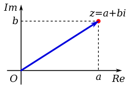
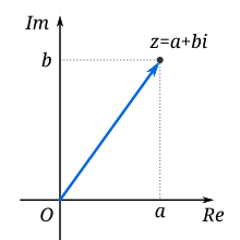
Изучение выше мы начали с алгебраической формы. Так как она является основополагающей. Чтобы было понятно в этой же форме изобразим комплексное число на плоскости:
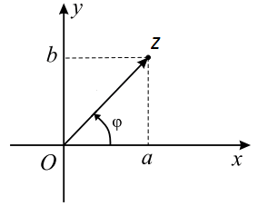 Видим, что $ a,b in mathbb{R} $ расположены на соответствующих осях плоскости.
Комплексное число $ z = a+ib $ представляется в виде вектора $ overline{z} $.
Аргумент обозначается $ varphi $.
Модуль $ |z| $ равняется длине вектора $ overline{z} $ и находится по формуле $ |z| = sqrt{a^2+b^2} $
Аргумент комплексного числа $ varphi $ нужно находить по различным формулам в зависимости от полуплоскости, в которой лежит само число.
Если:
- $ a>0 $, то $ varphi = arctgfrac{b}{a} $
- $ a<0, b>0 $, то $ varphi = pi + arctgfrac{b}{a} $
- $ a<0, b<0 $, то $ varphi = -pi + arctgfrac{b}{a} $
Операции
Над комплексными числами можно проводить различные операции, а именно:
- Складывать и вычитать
- Умножать и делить
- Извлекать корни и возводить в степень
- Переводить из одной формы в другую
Для нахождения суммы и разности складывается и вычитаются только соответствующие друг другу члены. Мнимая часть только с мнимой, а действительная только с действительной:
$$ z_1 + z_2 = (a_1+ib_1) + (a_2+ib_2) = (a_1 + a_2)+i(b_1 + b_2) $$
$$ z_1 — z_2 = (a_1+ib_1) — (a_2+ib_2) = (a_1 — a_2)+i(b_1 — b_2) $$
Умножение в алгебраической форме:
$$ z_1 cdot z_2 = (a_1+ib_1) cdot (a_2+ib_2) = (a_1 a_2 — b_1 b_2)+i(a_1 b_2 + a_2 b_1) $$
Умножение в показательной форме:
$$ z_1 cdot z_2 = |z_1|e^{ivarphi_1} cdot |z_2|e^{ivarphi_2} = |z_1|cdot|z_2|cdot e^{i(varphi_1 + varphi_2)} $$
Деление в алгебраической форме:
$$ frac{z_1}{z_2} = frac{a_1+ib_1}{a_2+ib_2} = frac{a_1 a_2 + b_1 b_2 }{a_2 ^2 + b_2 ^2} + i frac{a_2 b_1 — a_1 b_2}{a_2 ^2 + b_2 ^2} $$
Деление в показательной форме:
$$ frac{z_1}{z_2} = frac{|z_1|e^{ivarphi_1}}{|z_2|e^{ivarphi_2}} = frac{|z_1|}{|z_2|}e^{i(varphi_1 — varphi_2)} $$
Для возведения в степень необходимо умножить комплексное число само на себя необходимое количество раз, либо воспользоваться формулой Муавра:
$$ z^n = |z|^n(cos nvarphi+isin nvarphi) $$
Для извлечения корней необходимо также воспользоваться формулой Муавра:
$$ z^frac{1}{n} = |z|^frac{1}{n}bigg(cos frac{varphi + 2pi k}{n}+isin frac{varphi + 2pi k}{n}bigg), k=0,1,…,n-1 $$
Так же теория комплексных чисел помогает находить корни многочленов. Например, в квадратном уравнении, если $ D<0 $, то вещественных корней нет, но есть комплексные. В последнем примере рассмотрен данный случай.
Рассмотрим на практике комплексные числа: примеры с решением.
Примеры с решением
| Пример 1 |
| Перевести из алгебраической в тригонометрическую и показательную форму:$$ z = 4-4i $$ |
| Решение |
|
Для начала приступим к нахождению модуля комплексного числа: $$ |z| = sqrt{4^2 + (-4)^2} = sqrt{16 + 16} = sqrt{32} = 4sqrt{2} $$ Осталось найти аргумент: $$ varphi = arctg frac{b}{a} = arctg frac{-4}{4} = arctg (-1) = -frac{pi}{4} $$ Теперь составляем тригонометрическую запись комплексного числа, указанного в условии примера: $$ z = 4sqrt{2}bigg(sin(-frac{pi}{4}) + isin(-frac{pi}{4}) bigg) $$ Тут же можно записать показательную форму: $$ z = 4sqrt{2} e^{-frac{pi}{4}i} $$ Если не получается решить свою задачу, то присылайте её к нам. Мы предоставим подробное решение. Вы сможете ознакомиться с ходом вычисления и почерпнуть информацию. Это поможет своевременно получить зачёт у преподавателя! |
| Ответ |
|
$$ z = 4sqrt{2}bigg(sin(-frac{pi}{4}) + isin(-frac{pi}{4}) bigg) $$ $$ z = 4sqrt{2} e^{-frac{pi}{4}i} $$ |
| Пример 2 |
|
Вычислить сумму и разность заданных комплексных чисел: $$ z_1 = 3+i, z_2 = 5-2i $$ |
| Решение |
|
Сначала выполним сложение. Для этого просуммируем соответствующие мнимые и вещественные части комплексных чисел: $$ z_1 + z_2 = (3+i) + (5-2i) = (3+5)+(i-2i) = 8 — i $$ Аналогично выполним вычитание чисел: $$ z_1 — z_2 = (3+i) — (5-2i) = (3-5)+(i+2i) = -2 + 3i $$ |
| Ответ |
| $$ z_1 + z_2 = 8 — i; z_1 — z_2 = -2 + 3i $$ |
| Пример 3 |
|
Выполнить умножение и деление комплексных чисел: $$ z_1 = 3+i, z_2 = 5-2i $$ |
| Решение |
|
$$ z_1 cdot z_2 = (3+i) cdot (5-2i) = $$ Просто на просто раскроем скобки и произведем приведение подобных слагаемых, так же учтем, что $ i^2 = -1 $: $$ = 15 — 6i + 5i -2i^2 = 15 — i — 2cdot(-1) = $$ $$ = 15 — i + 2 = 17 — i $$ Так, теперь разделим первое число на второе: $$ frac{z_1}{z_2} = frac{3+i}{5-2i} = $$ Суть деления в том, чтобы избавиться от комплексного числа в знаменателе. Для этого нужно домножить числитель и знаменатель дроби на комплексно-сопряженное число к знаменателю и затем раскрываем все скобки: $$ = frac{(3+i)(5+2i)}{(5-2i)(5+2i)} = frac{15 + 6i + 5i + 2i^2}{25 + 10i — 10i -4i^2} = $$ $$ = frac{15 + 11i -2}{25 + 4} = frac{13 + 11i}{29} $$ Разделим числитель на 29, чтобы записать дробь в виде алгебраической формы: $$ frac{z_1}{z_2} = frac{13}{29} + frac{11}{29}i $$ |
| Ответ |
| $$ z_1 cdot z_2 = 17 — i; frac{z_1}{z_2} = frac{13}{29} + frac{11}{29}i $$ |
| Пример 4 |
| Возвести комплексное число $ z = 3+3i $ в степень: a) $ n=2 $ б) $ n=7 $ |
| Решение |
|
1) $ n = 2 $ Для возведения в квадрат достаточно умножить число само на себя: $$ z^2 = (3+3i)^2 = (3+3i)cdot (3+3i) = $$ Пользуемся формулой для умножения, раскрываем скобки и приводим подобные: $$ =9 + 9i + 3icdot 3 + 9i^2 = 9 + 18i — 9 = 18i $$ Получили ответ, что $$ z^2 = (3+i)^2 = 18i $$ 2) $ n = 7 $ В этом случае не всё так просто как в предыдущем случае, когда было возведение в квадрат. Конечно, можно прибегнуть к способу озвученному ранее и умножить число само на себя 7 раз, но это будет очень долгое и длинное решение. Гораздо проще будет воспользоваться формулой Муавра. Но она работает с числами в тригонометрической форме, а число задано в алгебраической. Значит, прежде переведем из одной формы в другую. Вычисляем значение модуля: $$ |z| = sqrt{3^2 + 3^2} = sqrt{9 + 9} = sqrt{18} = 3sqrt{2} $$ Найдем чем равен аргумент: $$ varphi = arctg frac{3}{3} = arctg(1) = frac{pi}{4} $$ Записываем в тригонометрическом виде: $$ z = 3sqrt{2}(cos frac{pi}{4} + isin frac{pi}{4}) $$ Возводим в степень $ n = 7 $: $$ z^7 = (3sqrt{2})^7 (cos frac{7pi}{4} + isin frac{7pi}{4}) = $$ Преобразуем в алгебраическую форму для наглядности: $$ =(3sqrt{2})^7 (frac{1}{sqrt{2}}-ifrac{1}{sqrt{2}}) = $$ $$ = 3^7 sqrt{2}^7 (frac{1}{sqrt{2}}-ifrac{1}{sqrt{2}}) = $$ $$ = 3^7 sqrt{2}^6 (1-i) = 3^7 cdot 8(1-i) = $$ $$ = 2187 cdot 8 (1-i) = 17496(1-i) $$ |
| Ответ |
|
$$ z^2 = (3+i)^2 = 18i $$ $$ z^7 = 17496(1-i) $$ |
| Пример 5 |
| Извлечь корень $ sqrt[3]{-1} $ над множеством $ mathbb{C} $ |
| Решение |
|
Представим число в тригонометрической форме. Найдем модуль и аргумент: $$ |z| = sqrt{(-1)^2 + 0^2} = sqrt{1+0} = sqrt{1}=1 $$ $$ varphi = arctg frac{0}{-1} +pi = arctg 0 + pi = pi $$ Получаем: $$ z = (cos pi + isin pi) $$ Используем знакомую формулу Муавра для вычисления корней любой степени: $$ z^frac{1}{n} = r^frac{1}{n}bigg(cos frac{varphi + 2pi k}{n}+isin frac{varphi + 2pi k}{n}bigg), k=0,1,…,n-1 $$ Так как степень $ n = 3 $, то по формуле $ k = 0,1,2 $: $$ z_0 = sqrt[3]{1} (cos frac{pi}{3}+isin frac{pi}{3}) = frac{1}{2}+ifrac{sqrt{3}}{2} $$ $$ z_1 = sqrt[3]{1} (cos frac{3pi}{3}+isin frac{3pi}{3}) = -1 $$ $$ z_2 = sqrt[3]{1} (cos frac{5pi}{3}+isin frac{5pi}{3}) = frac{1}{2} — ifrac{sqrt{3}}{2} $$ |
| Ответ |
|
$$ z_0 = frac{1}{2}+ifrac{sqrt{3}}{2} $$ $$ z_1 = -1 $$ $$ z_2 = frac{1}{2} — ifrac{sqrt{3}}{2} $$ |
| Пример 6 |
| Решить квадратное уравнение $ x^2 + 2x + 2 = 0 $ над $ mathbb{C} $ |
| Решение |
|
Решать будем по общей формуле, которую все выучили в 8 классе. Находим дискриминант $$ D = b^2 — 4ac = 2^2 — 4cdot 1 cdot 2 = 4-8 = -4 $$ Получили, что $ D=-4<0 $ и казалось бы, что решение можно заканчивать. Но нет! В нашем задании требуется решить уравнение над комплексным множеством, а то что дискриминант отрицательный означает только лишь отсутствие вещественных корней. А комплексные корни есть! Найдем их продолжив решение: $$ x_{1,2} = frac{-bpm sqrt{D}}{2a} = frac{-2pm sqrt{-4}}{2} = $$ Заметим, что $ sqrt{-4} = 2sqrt{-1} = 2i $ и продолжим вычисление: $$ = frac{-2 pm 2i}{2} = -1 pm i $$ Получили комплексно-сопряженные корни: $$ x_1 = -1 — i; x_2 = -1 — i $$ Как видите любой многочлен можно решить благодаря комплексным числам. |
| Ответ |
| $$ x_1 = -1 — i; x_2 = -1 — i $$ |
В статье «Комплексные числа: примеры с решением» было дано определение, основные понятия, формы записи, алгебраические операции и решение практических примеров.
Напомним необходимые сведения о комплексных числах.
Комплексное число — это выражение вида a + bi, где a, b — действительные числа, а i — так называемая мнимая единица, символ, квадрат которого равен –1, то есть i2 = –1. Число a называется действительной частью, а число b — мнимой частью комплексного числа z = a + bi. Если b = 0, то вместо a + 0i пишут просто a. Видно, что действительные числа — это частный случай комплексных чисел.
Арифметические действия над комплексными числами те же, что и над действительными: их можно складывать, вычитать, умножать и делить друг на друга. Сложение и вычитание происходят по правилу (a + bi) ± (c + di) = (a ± c) + (b ± d)i, а умножение — по правилу (a + bi) · (c + di) = (ac – bd) + (ad + bc)i (здесь как раз используется, что i2 = –1). Число ![]() = a – bi называется комплексно-сопряженным к z = a + bi. Равенство z ·
= a – bi называется комплексно-сопряженным к z = a + bi. Равенство z · ![]() = a2 + b2 позволяет понять, как делить одно комплексное число на другое (ненулевое) комплексное число:
= a2 + b2 позволяет понять, как делить одно комплексное число на другое (ненулевое) комплексное число:
![]() .
.
(Например, ![]() .)
.)

У комплексных чисел есть удобное и наглядное геометрическое представление: число z = a + bi можно изображать вектором с координатами (a; b) на декартовой плоскости (или, что почти то же самое, точкой — концом вектора с этими координатами). При этом сумма двух комплексных чисел изображается как сумма соответствующих векторов (которую можно найти по правилу параллелограмма). По теореме Пифагора длина вектора с координатами (a; b) равна ![]() . Эта величина называется модулем комплексного числа z = a + bi и обозначается |z|. Угол, который этот вектор образует с положительным направлением оси абсцисс (отсчитанный против часовой стрелки), называется аргументом комплексного числа z и обозначается Arg z. Аргумент определен не однозначно, а лишь с точностью до прибавления величины, кратной 2π радиан (или 360°, если считать в градусах) — ведь ясно, что поворот на такой угол вокруг начала координат не изменит вектор. Но если вектор длины r образует угол φ с положительным направлением оси абсцисс, то его координаты равны (r · cos φ; r · sin φ). Отсюда получается тригонометрическая форма записи комплексного числа: z = |z| · (cos(Arg z) + i sin(Arg z)). Часто бывает удобно записывать комплексные числа именно в такой форме, потому что это сильно упрощает выкладки. Умножение комплексных чисел в тригонометрической форме выглядит очень просто: z1 · z2 = |z1| · |z2| · (cos(Arg z1 + Arg z2) + i sin(Arg z1 + Arg z2)) (при умножении двух комплексных чисел их модули перемножаются, а аргументы складываются). Отсюда следуют формулы Муавра: zn = |z|n · (cos(n · (Arg z)) + i sin(n · (Arg z))). С помощью этих формул легко научиться извлекать корни любой степени
. Эта величина называется модулем комплексного числа z = a + bi и обозначается |z|. Угол, который этот вектор образует с положительным направлением оси абсцисс (отсчитанный против часовой стрелки), называется аргументом комплексного числа z и обозначается Arg z. Аргумент определен не однозначно, а лишь с точностью до прибавления величины, кратной 2π радиан (или 360°, если считать в градусах) — ведь ясно, что поворот на такой угол вокруг начала координат не изменит вектор. Но если вектор длины r образует угол φ с положительным направлением оси абсцисс, то его координаты равны (r · cos φ; r · sin φ). Отсюда получается тригонометрическая форма записи комплексного числа: z = |z| · (cos(Arg z) + i sin(Arg z)). Часто бывает удобно записывать комплексные числа именно в такой форме, потому что это сильно упрощает выкладки. Умножение комплексных чисел в тригонометрической форме выглядит очень просто: z1 · z2 = |z1| · |z2| · (cos(Arg z1 + Arg z2) + i sin(Arg z1 + Arg z2)) (при умножении двух комплексных чисел их модули перемножаются, а аргументы складываются). Отсюда следуют формулы Муавра: zn = |z|n · (cos(n · (Arg z)) + i sin(n · (Arg z))). С помощью этих формул легко научиться извлекать корни любой степени  из комплексных чисел. Корень n-й степени из числа z — это такое комплексное число w, что wn = z. Видно, что
 ![]() , а
, а ![]() , где k может принимать любое значение из множества {0, 1, …, n – 1}. Это означает, что всегда есть ровно n корней n-й степени из комплексного числа (на плоскости они располагаются в вершинах правильного n-угольника).
, где k может принимать любое значение из множества {0, 1, …, n – 1}. Это означает, что всегда есть ровно n корней n-й степени из комплексного числа (на плоскости они располагаются в вершинах правильного n-угольника).
Далее: Фрактальные размерности
A complex number can be visually represented as a pair of numbers (a, b) forming a vector on a diagram called an Argand diagram, representing the complex plane. Re is the real axis, Im is the imaginary axis, and i is the «imaginary unit», that satisfies i2 = −1.
In mathematics, a complex number is an element of a number system that extends the real numbers with a specific element denoted i, called the imaginary unit and satisfying the equation  ; every complex number can be expressed in the form
  , where a and b are real numbers. Because no real number satisfies the above equation, i was called an imaginary number by René Descartes. For the complex number , a is called the real part, and b is called the imaginary part. The set of complex numbers is denoted by either of the symbols
  or C. Despite the historical nomenclature «imaginary», complex numbers are regarded in the mathematical sciences as just as «real» as the real numbers and are fundamental in many aspects of the scientific description of the natural world.[1][a]
Complex numbers allow solutions to all polynomial equations, even those that have no solutions in real numbers. More precisely, the fundamental theorem of algebra asserts that every non-constant polynomial equation with real or complex coefficients has a solution which is a complex number. For example, the equation

has no real solution, since the square of a real number cannot be negative, but has the two nonreal complex solutions  and
and  .
.
Addition, subtraction and multiplication of complex numbers can be naturally defined by using the rule combined with the associative, commutative, and distributive laws. Every nonzero complex number has a multiplicative inverse. This makes the complex numbers a field that has the real numbers as a subfield. The complex numbers also form a real vector space of dimension two, with {1, i} as a standard basis.
This standard basis makes the complex numbers a Cartesian plane, called the complex plane. This allows a geometric interpretation of the complex numbers and their operations, and conversely expressing in terms of complex numbers some geometric properties and constructions. For example, the real numbers form the real line which is identified to the horizontal axis of the complex plane. The complex numbers of absolute value one form the unit circle. The addition of a complex number is a translation in the complex plane, and the multiplication by a complex number is a similarity centered at the origin. The complex conjugation is the reflection symmetry with respect to the real axis. The complex absolute value is a Euclidean norm.
In summary, the complex numbers form a rich structure that is simultaneously an algebraically closed field, a commutative algebra over the reals, and a Euclidean vector space of dimension two.
Definition[edit]

An illustration of the complex number z = x + iy on the complex plane. The real part is x, and its imaginary part is y.
A complex number is a number of the form a + bi, where a and b are real numbers, and i is an indeterminate satisfying i2 = −1. For example, 2 + 3i is a complex number.[3]
This way, a complex number is defined as a polynomial with real coefficients in the single indeterminate i, for which the relation i2 + 1 = 0 is imposed. Based on this definition, complex numbers can be added and multiplied, using the addition and multiplication for polynomials. The relation i2 + 1 = 0 induces the equalities i4k = 1, i4k+1 = i, i4k+2 = −1, and i4k+3 = −i, which hold for all integers k; these allow the reduction of any polynomial that results from the addition and multiplication of complex numbers to a linear polynomial in i, again of the form a + bi with real coefficients a, b.
The real number a is called the real part of the complex number a + bi; the real number b is called its imaginary part. To emphasize, the imaginary part does not include a factor i; that is, the imaginary part is b, not bi.[4][5]
Formally, the complex numbers are defined as the quotient ring of the polynomial ring in the indeterminate i, by the ideal generated by the polynomial i2 + 1 (see below).[6]
Notation[edit]
A real number a can be regarded as a complex number a + 0i, whose imaginary part is 0. A purely imaginary number bi is a complex number 0 + bi, whose real part is zero. As with polynomials, it is common to write a for a + 0i and bi for 0 + bi. Moreover, when the imaginary part is negative, that is, b = −|b| < 0, it is common to write a − |b|i instead of a + (−|b|)i; for example, for b = −4, 3 − 4i can be written instead of 3 + (−4)i.
Since the multiplication of the indeterminate i and a real is commutative in polynomials with real coefficients, the polynomial a + bi may be written as a + ib. This is often expedient for imaginary parts denoted by expressions, for example, when b is a radical.[7]
The real part of a complex number z is denoted by Re(z),  , or
, or  ; the imaginary part of a complex number z is denoted by Im(z),
  , or
, or  For example,

The set of all complex numbers is denoted by (blackboard bold) or C (upright bold).
In some disciplines, particularly in electromagnetism and electrical engineering, j is used instead of i as i is frequently used to represent electric current.[8] In these cases, complex numbers are written as a + bj, or a + jb.
Visualization[edit]
A complex number z, as a point (black) and its position vector (blue)
A complex number z can thus be identified with an ordered pair  of real numbers, which in turn may be interpreted as coordinates of a point in a two-dimensional space. The most immediate space is the Euclidean plane with suitable coordinates, which is then called complex plane or Argand diagram,[9][b][10] named after Jean-Robert Argand. Another prominent space on which the coordinates may be projected is the two-dimensional surface of a sphere, which is then called Riemann sphere.
Cartesian complex plane[edit]
The definition of the complex numbers involving two arbitrary real values immediately suggests the use of Cartesian coordinates in the complex plane. The horizontal (real) axis is generally used to display the real part, with increasing values to the right, and the imaginary part marks the vertical (imaginary) axis, with increasing values upwards.
A charted number may be viewed either as the coordinatized point or as a position vector from the origin to this point. The coordinate values of a complex number z can hence be expressed in its Cartesian, rectangular, or algebraic form.
Notably, the operations of addition and multiplication take on a very natural geometric character, when complex numbers are viewed as position vectors: addition corresponds to vector addition, while multiplication (see below) corresponds to multiplying their magnitudes and adding the angles they make with the real axis. Viewed in this way, the multiplication of a complex number by i corresponds to rotating the position vector counterclockwise by a quarter turn (90°) about the origin—a fact which can be expressed algebraically as follows:

Polar complex plane [edit]
«Polar form» redirects here. For the higher-dimensional analogue, see Polar decomposition.
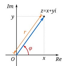
Argument φ and modulus r locate a point in the complex plane.
Modulus and argument[edit]
An alternative option for coordinates in the complex plane is the polar coordinate system that uses the distance of the point z from the origin (O), and the angle subtended between the positive real axis and the line segment Oz in a counterclockwise sense. This leads to the polar form

of a complex number, where r is the absolute value of z, and  is the argument of z.
The absolute value (or modulus or magnitude) of a complex number z = x + yi is[11]

If z is a real number (that is, if y = 0), then r = |x|. That is, the absolute value of a real number equals its absolute value as a complex number.
By Pythagoras’ theorem, the absolute value of a complex number is the distance to the origin of the point representing the complex number in the complex plane.
The argument of z (in many applications referred to as the «phase» φ)[10] is the angle of the radius Oz with the positive real axis, and is written as arg z. As with the modulus, the argument can be found from the rectangular form x + yi[12]—by applying the inverse tangent to the quotient of imaginary-by-real parts. By using a half-angle identity, a single branch of the arctan suffices to cover the range (−π, π] of the arg-function, and avoids a more subtle case-by-case analysis

Normally, as given above, the principal value in the interval (−π, π] is chosen. If the arg value is negative, values in the range (−π, π] or [0, 2π) can be obtained by adding 2π. The value of φ is expressed in radians in this article. It can increase by any integer multiple of 2π and still give the same angle, viewed as subtended by the rays of the positive real axis and from the origin through z. Hence, the arg function is sometimes considered as multivalued. The polar angle for the complex number 0 is indeterminate, but arbitrary choice of the polar angle 0 is common.
The value of φ equals the result of atan2:

Together, r and φ give another way of representing complex numbers, the polar form, as the combination of modulus and argument fully specify the position of a point on the plane. Recovering the original rectangular co-ordinates from the polar form is done by the formula called trigonometric form

Using Euler’s formula this can be written as

Using the cis function, this is sometimes abbreviated to

In angle notation, often used in electronics to represent a phasor with amplitude r and phase φ, it is written as[13]

Complex graphs[edit]
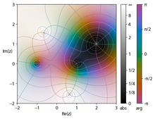
A color wheel graph of the expression (z2 − 1)(z − 2 − i)2/z2 + 2 + 2i
When visualizing complex functions, both a complex input and output are needed. Because each complex number is represented in two dimensions, visually graphing a complex function would require the perception of a four dimensional space, which is possible only in projections. Because of this, other ways of visualizing complex functions have been designed.
In domain coloring the output dimensions are represented by color and brightness, respectively. Each point in the complex plane as domain is ornated, typically with color representing the argument of the complex number, and brightness representing the magnitude. Dark spots mark moduli near zero, brighter spots are farther away from the origin, the gradation may be discontinuous, but is assumed as monotonous. The colors often vary in steps of π/3 for 0 to 2π from red, yellow, green, cyan, blue, to magenta. These plots are called color wheel graphs. This provides a simple way to visualize the functions without losing information. The picture shows zeros for ±1, (2 + i) and poles at 
History[edit]
The solution in radicals (without trigonometric functions) of a general cubic equation, when all three of its roots are real numbers, contains the square roots of negative numbers, a situation that cannot be rectified by factoring aided by the rational root test, if the cubic is irreducible; this is the so-called casus irreducibilis («irreducible case»). This conundrum led Italian mathematician Gerolamo Cardano to conceive of complex numbers in around 1545 in his Ars Magna,[14] though his understanding was rudimentary; moreover he later dismissed complex numbers as «subtle as they are useless».[15] Cardano did use imaginary numbers, but described using them as “mental torture.” [16] This was prior to the use of the graphical complex plane. Cardano and other Italian mathematicians, notably Scipione del Ferro, in the 1500s created an algorithm for solving cubic equations which generally had one real solution and two solutions containing an imaginary number. Since they ignored the answers with the imaginary numbers, Cardano found them useless.[17]
Work on the problem of general polynomials ultimately led to the fundamental theorem of algebra, which shows that with complex numbers, a solution exists to every polynomial equation of degree one or higher. Complex numbers thus form an algebraically closed field, where any polynomial equation has a root.
Many mathematicians contributed to the development of complex numbers. The rules for addition, subtraction, multiplication, and root extraction of complex numbers were developed by the Italian mathematician Rafael Bombelli.[18] A more abstract formalism for the complex numbers was further developed by the Irish mathematician William Rowan Hamilton, who extended this abstraction to the theory of quaternions.[19]
The earliest fleeting reference to square roots of negative numbers can perhaps be said to occur in the work of the Greek mathematician Hero of Alexandria in the 1st century AD, where in his Stereometrica he considered, apparently in error, the volume of an impossible frustum of a pyramid to arrive at the term  in his calculations, which today would simplify to
  . Negative quantities were not conceived of in Hellenistic mathematics and Hero merely replaced it by its positive
  [20]
[20]
The impetus to study complex numbers as a topic in itself first arose in the 16th century when algebraic solutions for the roots of cubic and quartic polynomials were discovered by Italian mathematicians (see Niccolò Fontana Tartaglia, Gerolamo Cardano). It was soon realized (but proved much later)[21] that these formulas, even if one were interested only in real solutions, sometimes required the manipulation of square roots of negative numbers. As an example, Tartaglia’s formula for a cubic equation of the form x3 = px + q[c] gives the solution to the equation x3 = x as

At first glance this looks like nonsense. However, formal calculations with complex numbers show that the equation z3 = i has three solutions:  Substituting these in turn for
  in Tartaglia’s cubic formula and simplifying, one gets 0, 1 and −1 as the solutions of x3 − x = 0. Of course this particular equation can be solved at sight but it does illustrate that when general formulas are used to solve cubic equations with real roots then, as later mathematicians showed rigorously,[d] the use of complex numbers is unavoidable. Rafael Bombelli was the first to address explicitly these seemingly paradoxical solutions of cubic equations and developed the rules for complex arithmetic trying to resolve these issues.
The term «imaginary» for these quantities was coined by René Descartes in 1637, who was at pains to stress their unreal nature[22]
… sometimes only imaginary, that is one can imagine as many as I said in each equation, but sometimes there exists no quantity that matches that which we imagine.
[… quelquefois seulement imaginaires c’est-à-dire que l’on peut toujours en imaginer autant que j’ai dit en chaque équation, mais qu’il n’y a quelquefois aucune quantité qui corresponde à celle qu’on imagine.]
A further source of confusion was that the equation  seemed to be capriciously inconsistent with the algebraic identity
  , which is valid for non-negative real numbers a and b, and which was also used in complex number calculations with one of a, b positive and the other negative. The incorrect use of this identity (and the related identity
  ) in the case when both a and b are negative even bedeviled Leonhard Euler. This difficulty eventually led to the convention of using the special symbol i in place of
  to guard against this mistake.[citation needed] Even so, Euler considered it natural to introduce students to complex numbers much earlier than we do today. In his elementary algebra text book, Elements of Algebra, he introduces these numbers almost at once and then uses them in a natural way throughout.
In the 18th century complex numbers gained wider use, as it was noticed that formal manipulation of complex expressions could be used to simplify calculations involving trigonometric functions. For instance, in 1730 Abraham de Moivre noted that the identities relating trigonometric functions of an integer multiple of an angle to powers of trigonometric functions of that angle could be re-expressed by the following de Moivre’s formula:

In 1748, Euler went further and obtained Euler’s formula of complex analysis:[23]

by formally manipulating complex power series and observed that this formula could be used to reduce any trigonometric identity to much simpler exponential identities.
The idea of a complex number as a point in the complex plane (above) was first described by Danish–Norwegian mathematician Caspar Wessel in 1799,[24] although it had been anticipated as early as 1685 in Wallis’s A Treatise of Algebra.[25]
Wessel’s memoir appeared in the Proceedings of the Copenhagen Academy but went largely unnoticed. In 1806 Jean-Robert Argand independently issued a pamphlet on complex numbers and provided a rigorous proof of the fundamental theorem of algebra.[26] Carl Friedrich Gauss had earlier published an essentially topological proof of the theorem in 1797 but expressed his doubts at the time about «the true metaphysics of the square root of −1».[27] It was not until 1831 that he overcame these doubts and published his treatise on complex numbers as points in the plane,[28] largely establishing modern notation and terminology:[29]
If one formerly contemplated this subject from a false point of view and therefore found a mysterious darkness, this is in large part attributable to clumsy terminology. Had one not called +1, -1,
positive, negative, or imaginary (or even impossible) units, but instead, say, direct, inverse, or lateral units, then there could scarcely have been talk of such darkness.
In the beginning of the 19th century, other mathematicians discovered independently the geometrical representation of the complex numbers: Buée,[30][31] Mourey,[32] Warren,[33][34][35] Français and his brother, Bellavitis.[36][37]
The English mathematician G.H. Hardy remarked that Gauss was the first mathematician to use complex numbers in ‘a really confident and scientific way’ although mathematicians such as Norwegian Niels Henrik Abel and Carl Gustav Jacob Jacobi were necessarily using them routinely before Gauss published his 1831 treatise.[38]
Augustin-Louis Cauchy and Bernhard Riemann together brought the fundamental ideas of complex analysis to a high state of completion, commencing around 1825 in Cauchy’s case.
The common terms used in the theory are chiefly due to the founders. Argand called cos φ + i sin φ the direction factor, and  the modulus;[e][39] Cauchy (1821) called cos φ + i sin φ the reduced form (l’expression réduite)[40] and apparently introduced the term argument; Gauss used i for ,[f] introduced the term complex number for a + bi,[g] and called a2 + b2 the norm.[h] The expression direction coefficient, often used for cos φ + i sin φ, is due to Hankel (1867),[44] and absolute value, for modulus, is due to Weierstrass.
Later classical writers on the general theory include Richard Dedekind, Otto Hölder, Felix Klein, Henri Poincaré, Hermann Schwarz, Karl Weierstrass and many others. Important work (including a systematization) in complex multivariate calculus has been started at beginning of the 20th century. Important results have been achieved by Wilhelm Wirtinger in 1927.
Relations and operations[edit]
Equality[edit]
Complex numbers have a similar definition of equality to real numbers; two complex numbers a1 + b1i and a2 + b2i are equal if and only if both their real and imaginary parts are equal, that is, if a1 = a2 and b1 = b2. Nonzero complex numbers written in polar form are equal if and only if they have the same magnitude and their arguments differ by an integer multiple of 2π.
Ordering[edit]
Unlike the real numbers, there is no natural ordering of the complex numbers. In particular, there is no linear ordering on the complex numbers that is compatible with addition and multiplication. Hence, the complex numbers do not have the structure of an ordered field. One explanation for this is that every non-trivial sum of squares in an ordered field is nonzero, and i2 + 12 = 0 is a non-trivial sum of squares. Thus, complex numbers are naturally thought of as existing on a two-dimensional plane.
Conjugate[edit]

Geometric representation of z and its conjugate z in the complex plane
The complex conjugate of the complex number z = x + yi is given by x − yi. It is denoted by either z or z*.[45] This unary operation on complex numbers cannot be expressed by applying only their basic operations addition, subtraction, multiplication and division.
Geometrically, z is the «reflection» of z about the real axis. Conjugating twice gives the original complex number

which makes this operation an involution. The reflection leaves both the real part and the magnitude of z unchanged, that is

and 
The imaginary part and the argument of a complex number z change their sign under conjugation

For details on argument and magnitude, see the section on Polar form.
The product of a complex number z = x + yi and its conjugate is known as the absolute square. It is always a non-negative real number and equals the square of the magnitude of each:

This property can be used to convert a fraction with a complex denominator to an equivalent fraction with a real denominator by expanding both numerator and denominator of the fraction by the conjugate of the given denominator. This process is sometimes called «rationalization» of the denominator (although the denominator in the final expression might be an irrational real number), because it resembles the method to remove roots from simple expressions in a denominator.
The real and imaginary parts of a complex number z can be extracted using the conjugation:

Moreover, a complex number is real if and only if it equals its own conjugate.
Conjugation distributes over the basic complex arithmetic operations:

Conjugation is also employed in inversive geometry, a branch of geometry studying reflections more general than ones about a line. In the network analysis of electrical circuits, the complex conjugate is used in finding the equivalent impedance when the maximum power transfer theorem is looked for.
Addition and subtraction[edit]

Addition of two complex numbers can be done geometrically by constructing a parallelogram.
Two complex numbers  and
and  are most easily added by separately adding their real and imaginary parts. That is to say:

Similarly, subtraction can be performed as

Multiplication of a complex number and a real number r can be done similarly by multiplying separately r and the real and imaginary parts of a:

In particular, subtraction can be done by negating the subtrahend (that is multiplying it with –1) and adding the result to the minuend:

Using the visualization of complex numbers in the complex plane, addition has the following geometric interpretation: the sum of two complex numbers a and b, interpreted as points in the complex plane, is the point obtained by building a parallelogram from the three vertices O, and the points of the arrows labeled a and b (provided that they are not on a line). Equivalently, calling these points A, B, respectively and the fourth point of the parallelogram X the triangles OAB and XBA are congruent.
Multiplication and square[edit]
The rules of the distributive property, the commutative properties (of addition and multiplication), and the defining property i2 = −1 apply to complex numbers. It follows that

In particular,

Reciprocal and division[edit]
Using the conjugation, the reciprocal of a nonzero complex number z = x + yi can always be broken down to

since non-zero implies that x2 + y2 is greater than zero.
This can be used to express a division of an arbitrary complex number w = u + vi by a non-zero complex number z as

Multiplication and division in polar form[edit]
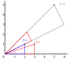
Multiplication of 2 + i (blue triangle) and 3 + i (red triangle). The red triangle is rotated to match the vertex of the blue one (the adding of both angles in the terms φ1+φ2 in the equation) and stretched by the length of the hypotenuse of the blue triangle (the multiplication of both radiuses, as per term r1r2 in the equation).
Formulas for multiplication, division and exponentiation are simpler in polar form than the corresponding formulas in Cartesian coordinates. Given two complex numbers z1 = r1(cos φ1 + i sin φ1) and z2 = r2(cos φ2 + i sin φ2), because of the trigonometric identities

we may derive

In other words, the absolute values are multiplied and the arguments are added to yield the polar form of the product. For example, multiplying by i corresponds to a quarter-turn counter-clockwise, which gives back i2 = −1. The picture at the right illustrates the multiplication of

Since the real and imaginary part of 5 + 5i are equal, the argument of that number is 45 degrees, or π/4 (in radian). On the other hand, it is also the sum of the angles at the origin of the red and blue triangles are arctan(1/3) and arctan(1/2), respectively. Thus, the formula

holds. As the arctan function can be approximated highly efficiently, formulas like this – known as Machin-like formulas – are used for high-precision approximations of π.
Similarly, division is given by

Square root[edit]
The square roots of a + bi (with b ≠ 0) are  , where

and

where sgn is the signum function. This can be seen by squaring to obtain a + bi.[46][47] Here  is called the modulus of a + bi, and the square root sign indicates the square root with non-negative real part, called the principal square root; also
  where z = a + bi.[48]
Exponential function[edit]
The exponential function  can be defined for every complex number z by the power series

which has an infinite radius of convergence.
The value at 1 of the exponential function is Euler’s number

If z is real, one has

Analytic continuation allows extending this equality for every complex value of z, and thus to define the complex exponentiation with base e as

Functional equation[edit]
The exponential function satisfies the functional equation 
This can be proved either by comparing the power series expansion of both members or by applying analytic continuation from the restriction of the equation to real arguments.
Euler’s formula[edit]
Euler’s formula states that, for any real number y,

The functional equation implies thus that, if x and y are real, one has

which is the decomposition of the exponential function into its real and imaginary parts.
Complex logarithm[edit]
In the real case, the natural logarithm can be defined as the inverse
 of the exponential function. For extending this to the complex domain, one can start from Euler’s formula. It implies that, if a complex number
  is written in polar form

with  then with

as complex logarithm one has a proper inverse:

However, because cosine and sine are periodic functions, the addition of an integer multiple of 2π to φ does not change z. For example, eiπ = e3iπ = −1 , so both iπ and 3iπ are possible values for the natural logarithm of −1.
Therefore, if the complex logarithm is not to be defined as a multivalued function

one has to use a branch cut and to restrict the codomain, resulting in the bijective function
![{displaystyle ln colon ;mathbb {C} ^{times };to ;;;mathbb {R} ^{+}+;i,left(-pi ,pi right].}](https://wikimedia.org/api/rest_v1/media/math/render/svg/5a9195ba0433fd0b1768386d0e3b2c11fb5eb684)
If  is not a non-positive real number (a positive or a non-real number), the resulting principal value of the complex logarithm is obtained with −π < φ < π. It is an analytic function outside the negative real numbers, but it cannot be prolongated to a function that is continuous at any negative real number
  , where the principal value is ln z = ln(−z) + iπ.[i]
Exponentiation[edit]
If x > 0 is real and z complex, the exponentiation is defined as

where ln denotes the natural logarithm.
It seems natural to extend this formula to complex values of x, but there are some difficulties resulting from the fact that the complex logarithm is not really a function, but a multivalued function.
It follows that if z is as above, and if t is another complex number, then the exponentiation is the multivalued function

Integer and fractional exponents[edit]

Geometric representation of the 2nd to 6th roots of a complex number z, in polar form reiφ where r = |z | and φ = arg z. If z is real, φ = 0 or π. Principal roots are shown in black.
If, in the preceding formula, t is an integer, then the sine and the cosine are independent of k. Thus, if the exponent n is an integer, then zn is well defined, and the exponentiation formula simplifies to de Moivre’s formula:

The n nth roots of a complex number z are given by
![{displaystyle z^{1/n}={sqrt[{n}]{r}}left(cos left({frac {varphi +2kpi }{n}}right)+isin left({frac {varphi +2kpi }{n}}right)right)}](https://wikimedia.org/api/rest_v1/media/math/render/svg/1cc1b3406644f788c1ac1799d6328118ee66516f)
for 0 ≤ k ≤ n − 1. (Here ![{displaystyle {sqrt[{n}]{r}}}](https://wikimedia.org/api/rest_v1/media/math/render/svg/10eb7386bd8efe4c5b5beafe05848fbd923e1413) is the usual (positive) nth root of the positive real number r.) Because sine and cosine are periodic, other integer values of k do not give other values.
is the usual (positive) nth root of the positive real number r.) Because sine and cosine are periodic, other integer values of k do not give other values.
While the nth root of a positive real number r is chosen to be the positive real number c satisfying cn = r, there is no natural way of distinguishing one particular complex nth root of a complex number. Therefore, the nth root is a n-valued function of z. This implies that, contrary to the case of positive real numbers, one has

since the left-hand side consists of n values, and the right-hand side is a single value.
Properties[edit]
Field structure[edit]
The set of complex numbers is a field.[49] Briefly, this means that the following facts hold: first, any two complex numbers can be added and multiplied to yield another complex number. Second, for any complex number z, its additive inverse –z is also a complex number; and third, every nonzero complex number has a reciprocal complex number. Moreover, these operations satisfy a number of laws, for example the law of commutativity of addition and multiplication for any two complex numbers z1 and z2:

These two laws and the other requirements on a field can be proven by the formulas given above, using the fact that the real numbers themselves form a field.
Unlike the reals, is not an ordered field, that is to say, it is not possible to define a relation z1 < z2 that is compatible with the addition and multiplication. In fact, in any ordered field, the square of any element is necessarily positive, so i2 = −1 precludes the existence of an ordering on  [50]
[50]
When the underlying field for a mathematical topic or construct is the field of complex numbers, the topic’s name is usually modified to reflect that fact. For example: complex analysis, complex matrix, complex polynomial, and complex Lie algebra.
Solutions of polynomial equations[edit]
Given any complex numbers (called coefficients) a0, …, an, the equation

has at least one complex solution z, provided that at least one of the higher coefficients a1, …, an is nonzero.[6] This is the statement of the fundamental theorem of algebra, of Carl Friedrich Gauss and Jean le Rond d’Alembert. Because of this fact, is called an algebraically closed field. This property does not hold for the field of rational numbers  (the polynomial x2 − 2 does not have a rational root, since √2 is not a rational number) nor the real numbers
  (the polynomial x2 + a does not have a real root for a > 0, since the square of x is positive for any real number x).
There are various proofs of this theorem, by either analytic methods such as Liouville’s theorem, or topological ones such as the winding number, or a proof combining Galois theory and the fact that any real polynomial of odd degree has at least one real root.
Because of this fact, theorems that hold for any algebraically closed field apply to For example, any non-empty complex square matrix has at least one (complex) eigenvalue.
Algebraic characterization[edit]
The field has the following three properties:
It can be shown that any field having these properties is isomorphic (as a field) to For example, the algebraic closure of the field  of the p-adic number also satisfies these three properties, so these two fields are isomorphic (as fields, but not as topological fields).[51] Also, is isomorphic to the field of complex Puiseux series. However, specifying an isomorphism requires the axiom of choice. Another consequence of this algebraic characterization is that contains many proper subfields that are isomorphic to .
Characterization as a topological field[edit]
The preceding characterization of describes only the algebraic aspects of That is to say, the properties of nearness and continuity, which matter in areas such as analysis and topology, are not dealt with. The following description of as a topological field (that is, a field that is equipped with a topology, which allows the notion of convergence) does take into account the topological properties. contains a subset P (namely the set of positive real numbers) of nonzero elements satisfying the following three conditions:
- P is closed under addition, multiplication and taking inverses.
- If x and y are distinct elements of P, then either x − y or y − x is in P.
- If S is any nonempty subset of P, then S + P = x + P for some x in
Moreover, has a nontrivial involutive automorphism x ↦ x* (namely the complex conjugation), such that x x* is in P for any nonzero x in
Any field F with these properties can be endowed with a topology by taking the sets B(x, p) = { y | p − (y − x)(y − x)* ∈ P } as a base, where x ranges over the field and p ranges over P. With this topology F is isomorphic as a topological field to
The only connected locally compact topological fields are and This gives another characterization of as a topological field, since can be distinguished from because the nonzero complex numbers are connected, while the nonzero real numbers are not.[52]
Formal construction[edit]
Construction as ordered pairs[edit]
William Rowan Hamilton introduced the approach to define the set of complex numbers[53] as the set  of ordered pairs (a, b) of real numbers, in which the following rules for addition and multiplication are imposed:[49]

It is then just a matter of notation to express (a, b) as a + bi.
Construction as a quotient field[edit]
Though this low-level construction does accurately describe the structure of the complex numbers, the following equivalent definition reveals the algebraic nature of more immediately. This characterization relies on the notion of fields and polynomials. A field is a set endowed with addition, subtraction, multiplication and division operations that behave as is familiar from, say, rational numbers. For example, the distributive law

must hold for any three elements x, y and z of a field. The set of real numbers does form a field. A polynomial p(X) with real coefficients is an expression of the form

where the a0, …, an are real numbers. The usual addition and multiplication of polynomials endows the set ![{displaystyle mathbb {R} [X]}](https://wikimedia.org/api/rest_v1/media/math/render/svg/16d740527b0b7f949b4bf9c9ce004134bb490b68) of all such polynomials with a ring structure. This ring is called the polynomial ring over the real numbers.
of all such polynomials with a ring structure. This ring is called the polynomial ring over the real numbers.
The set of complex numbers is defined as the quotient ring ![{displaystyle mathbb {R} [X]/(X^{2}+1).}](https://wikimedia.org/api/rest_v1/media/math/render/svg/c2d5e66358adeeb47fc3dce55f79c523e9798b03) [6] This extension field contains two square roots of −1, namely (the cosets of) X and −X, respectively. (The cosets of) 1 and X form a basis of
[6] This extension field contains two square roots of −1, namely (the cosets of) X and −X, respectively. (The cosets of) 1 and X form a basis of ![{displaystyle mathbb {R} [X]/(X^{2}+1)}](https://wikimedia.org/api/rest_v1/media/math/render/svg/4a9561fb97d235fa5d9d975ea50b9ac958058410) as a real vector space, which means that each element of the extension field can be uniquely written as a linear combination in these two elements. Equivalently, elements of the extension field can be written as ordered pairs (a, b) of real numbers. The quotient ring is a field, because X2 + 1 is irreducible over
as a real vector space, which means that each element of the extension field can be uniquely written as a linear combination in these two elements. Equivalently, elements of the extension field can be written as ordered pairs (a, b) of real numbers. The quotient ring is a field, because X2 + 1 is irreducible over  so the ideal it generates is maximal.
The formulas for addition and multiplication in the ring ![{displaystyle mathbb {R} [X],}](https://wikimedia.org/api/rest_v1/media/math/render/svg/44b5607f4e6eded005f2fbf81c70cfff7f26fb26) modulo the relation X2 = −1, correspond to the formulas for addition and multiplication of complex numbers defined as ordered pairs. So the two definitions of the field are isomorphic (as fields).
modulo the relation X2 = −1, correspond to the formulas for addition and multiplication of complex numbers defined as ordered pairs. So the two definitions of the field are isomorphic (as fields).
Accepting that is algebraically closed, since it is an algebraic extension of in this approach, is therefore the algebraic closure of 
Matrix representation of complex numbers[edit]
Complex numbers a + bi can also be represented by 2 × 2 matrices that have the form:

Here the entries a and b are real numbers. As the sum and product of two such matrices is again of this form, these matrices form a subring of the ring 2 × 2 matrices.
A simple computation shows that the map:

is a ring isomorphism from the field of complex numbers to the ring of these matrices. This isomorphism associates the square of the absolute value of a complex number with the determinant of the corresponding matrix, and the conjugate of a complex number with the transpose of the matrix.
The geometric description of the multiplication of complex numbers can also be expressed in terms of rotation matrices by using this correspondence between complex numbers and such matrices. The action of the matrix on a vector (x, y) corresponds to the multiplication of x + iy by a + ib. In particular, if the determinant is 1, there is a real number t such that the matrix has the form:

In this case, the action of the matrix on vectors and the multiplication by the complex number  are both the rotation of the angle t.
Complex analysis[edit]

Color wheel graph of sin(1/z). White parts inside refer to numbers having large absolute values.
The study of functions of a complex variable is known as complex analysis and has enormous practical use in applied mathematics as well as in other branches of mathematics. Often, the most natural proofs for statements in real analysis or even number theory employ techniques from complex analysis (see prime number theorem for an example). Unlike real functions, which are commonly represented as two-dimensional graphs, complex functions have four-dimensional graphs and may usefully be illustrated by color-coding a three-dimensional graph to suggest four dimensions, or by animating the complex function’s dynamic transformation of the complex plane.
Complex exponential and related functions[edit]
The notions of convergent series and continuous functions in (real) analysis have natural analogs in complex analysis. A sequence of complex numbers is said to converge if and only if its real and imaginary parts do. This is equivalent to the (ε, δ)-definition of limits, where the absolute value of real numbers is replaced by the one of complex numbers. From a more abstract point of view, , endowed with the metric

is a complete metric space, which notably includes the triangle inequality

for any two complex numbers z1 and z2.
Like in real analysis, this notion of convergence is used to construct a number of elementary functions: the exponential function exp z, also written ez, is defined as the infinite series

The series defining the real trigonometric functions sine and cosine, as well as the hyperbolic functions sinh and cosh, also carry over to complex arguments without change. For the other trigonometric and hyperbolic functions, such as tangent, things are slightly more complicated, as the defining series do not converge for all complex values. Therefore, one must define them either in terms of sine, cosine and exponential, or, equivalently, by using the method of analytic continuation.
Euler’s formula states:

for any real number φ, in particular

, which is Euler’s identity.
Unlike in the situation of real numbers, there is an infinitude of complex solutions z of the equation

for any complex number w ≠ 0. It can be shown that any such solution z – called complex logarithm of w – satisfies

where arg is the argument defined above, and ln the (real) natural logarithm. As arg is a multivalued function, unique only up to a multiple of 2π, log is also multivalued. The principal value of log is often taken by restricting the imaginary part to the interval (−π, π].
Complex exponentiation zω is defined as

and is multi-valued, except when ω is an integer. For ω = 1 / n, for some natural number n, this recovers the non-uniqueness of nth roots mentioned above.
Complex numbers, unlike real numbers, do not in general satisfy the unmodified power and logarithm identities, particularly when naïvely treated as single-valued functions; see failure of power and logarithm identities. For example, they do not satisfy

Both sides of the equation are multivalued by the definition of complex exponentiation given here, and the values on the left are a subset of those on the right.
Holomorphic functions[edit]
A function f: → is called holomorphic if it satisfies the Cauchy–Riemann equations. For example, any -linear map → can be written in the form

with complex coefficients a and b. This map is holomorphic if and only if b = 0. The second summand  is real-differentiable, but does not satisfy the Cauchy–Riemann equations.
Complex analysis shows some features not apparent in real analysis. For example, any two holomorphic functions f and g that agree on an arbitrarily small open subset of necessarily agree everywhere. Meromorphic functions, functions that can locally be written as f(z)/(z − z0)n with a holomorphic function f, still share some of the features of holomorphic functions. Other functions have essential singularities, such as sin(1/z) at z = 0.
Applications[edit]
Complex numbers have applications in many scientific areas, including signal processing, control theory, electromagnetism, fluid dynamics, quantum mechanics, cartography, and vibration analysis. Some of these applications are described below.
Geometry[edit]
Shapes[edit]
Three non-collinear points  in the plane determine the shape of the triangle
  . Locating the points in the complex plane, this shape of a triangle may be expressed by complex arithmetic as

The shape  of a triangle will remain the same, when the complex plane is transformed by translation or dilation (by an affine transformation), corresponding to the intuitive notion of shape, and describing similarity. Thus each triangle is in a similarity class of triangles with the same shape.[54]
Fractal geometry[edit]
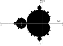
The Mandelbrot set with the real and imaginary axes labeled.
The Mandelbrot set is a popular example of a fractal formed on the complex plane. It is defined by plotting every location  where iterating the sequence
  does not diverge when iterated infinitely. Similarly, Julia sets have the same rules, except where remains constant.
Triangles[edit]
Every triangle has a unique Steiner inellipse – an ellipse inside the triangle and tangent to the midpoints of the three sides of the triangle. The foci of a triangle’s Steiner inellipse can be found as follows, according to Marden’s theorem:[55][56] Denote the triangle’s vertices in the complex plane as a = xA + yAi, b = xB + yBi, and c = xC + yCi. Write the cubic equation  , take its derivative, and equate the (quadratic) derivative to zero. Marden’s theorem says that the solutions of this equation are the complex numbers denoting the locations of the two foci of the Steiner inellipse.
Algebraic number theory[edit]

As mentioned above, any nonconstant polynomial equation (in complex coefficients) has a solution in . A fortiori, the same is true if the equation has rational coefficients. The roots of such equations are called algebraic numbers – they are a principal object of study in algebraic number theory. Compared to  , the algebraic closure of , which also contains all algebraic numbers, has the advantage of being easily understandable in geometric terms. In this way, algebraic methods can be used to study geometric questions and vice versa. With algebraic methods, more specifically applying the machinery of field theory to the number field containing roots of unity, it can be shown that it is not possible to construct a regular nonagon using only compass and straightedge – a purely geometric problem.
Another example is the Gaussian integers; that is, numbers of the form x + iy, where x and y are integers, which can be used to classify sums of squares.
Analytic number theory[edit]
Analytic number theory studies numbers, often integers or rationals, by taking advantage of the fact that they can be regarded as complex numbers, in which analytic methods can be used. This is done by encoding number-theoretic information in complex-valued functions. For example, the Riemann zeta function ζ(s) is related to the distribution of prime numbers.
Improper integrals[edit]
In applied fields, complex numbers are often used to compute certain real-valued improper integrals, by means of complex-valued functions. Several methods exist to do this; see methods of contour integration.
Dynamic equations[edit]
In differential equations, it is common to first find all complex roots r of the characteristic equation of a linear differential equation or equation system and then attempt to solve the system in terms of base functions of the form f(t) = ert. Likewise, in difference equations, the complex roots r of the characteristic equation of the difference equation system are used, to attempt to solve the system in terms of base functions of the form f(t) = rt.
Linear algebra[edit]
Eigendecomposition is a useful tool for computing matrix powers and matrix exponentials. However, it often requires the use of complex numbers, even if the matrix is real (for example, a rotation matrix).
Complex numbers often generalize concepts originally conceived in the real numbers. For example, the conjugate transpose generalizes the transpose, hermitian matrices generalize symmetric matrices, and unitary matrices generalize orthogonal matrices.
In applied mathematics[edit]
Control theory[edit]
In control theory, systems are often transformed from the time domain to the complex frequency domain using the Laplace transform. The system’s zeros and poles are then analyzed in the complex plane. The root locus, Nyquist plot, and Nichols plot techniques all make use of the complex plane.
In the root locus method, it is important whether zeros and poles are in the left or right half planes, that is, have real part greater than or less than zero. If a linear, time-invariant (LTI) system has poles that are
- in the right half plane, it will be unstable,
- all in the left half plane, it will be stable,
- on the imaginary axis, it will have marginal stability.
If a system has zeros in the right half plane, it is a nonminimum phase system.
Signal analysis[edit]
Complex numbers are used in signal analysis and other fields for a convenient description for periodically varying signals. For given real functions representing actual physical quantities, often in terms of sines and cosines, corresponding complex functions are considered of which the real parts are the original quantities. For a sine wave of a given frequency, the absolute value |z| of the corresponding z is the amplitude and the argument arg z is the phase.
If Fourier analysis is employed to write a given real-valued signal as a sum of periodic functions, these periodic functions are often written as complex-valued functions of the form

and

where ω represents the angular frequency and the complex number A encodes the phase and amplitude as explained above.
This use is also extended into digital signal processing and digital image processing, which use digital versions of Fourier analysis (and wavelet analysis) to transmit, compress, restore, and otherwise process digital audio signals, still images, and video signals.
Another example, relevant to the two side bands of amplitude modulation of AM radio, is:

In physics[edit]
Electromagnetism and electrical engineering[edit]
In electrical engineering, the Fourier transform is used to analyze varying voltages and currents. The treatment of resistors, capacitors, and inductors can then be unified by introducing imaginary, frequency-dependent resistances for the latter two and combining all three in a single complex number called the impedance. This approach is called phasor calculus.
In electrical engineering, the imaginary unit is denoted by j, to avoid confusion with I, which is generally in use to denote electric current, or, more particularly, i, which is generally in use to denote instantaneous electric current.
Since the voltage in an AC circuit is oscillating, it can be represented as

To obtain the measurable quantity, the real part is taken:
![{displaystyle v(t)=operatorname {Re} (V)=operatorname {Re} left[V_{0}e^{jomega t}right]=V_{0}cos omega t.}](https://wikimedia.org/api/rest_v1/media/math/render/svg/4b9078e78decc9fdf5d57a237bbf756b9cc438a0)
The complex-valued signal V(t) is called the analytic representation of the real-valued, measurable signal v(t).
[57]
Fluid dynamics[edit]
In fluid dynamics, complex functions are used to describe potential flow in two dimensions.
Quantum mechanics[edit]
The complex number field is intrinsic to the mathematical formulations of quantum mechanics, where complex Hilbert spaces provide the context for one such formulation that is convenient and perhaps most standard. The original foundation formulas of quantum mechanics – the Schrödinger equation and Heisenberg’s matrix mechanics – make use of complex numbers.
Relativity[edit]
In special and general relativity, some formulas for the metric on spacetime become simpler if one takes the time component of the spacetime continuum to be imaginary. (This approach is no longer standard in classical relativity, but is used in an essential way in quantum field theory.) Complex numbers are essential to spinors, which are a generalization of the tensors used in relativity.
Generalizations and related notions[edit]
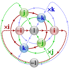
Cayley Q8 quaternion graph showing cycles of multiplication by i, j and k
The process of extending the field of reals to is known as the Cayley–Dickson construction. It can be carried further to higher dimensions, yielding the quaternions  and octonions
  which (as a real vector space) are of dimension 4 and 8, respectively.
In this context the complex numbers have been called the binarions.[58]
Just as by applying the construction to reals the property of ordering is lost, properties familiar from real and complex numbers vanish with each extension. The quaternions lose commutativity, that is, x·y ≠ y·x for some quaternions x, y, and the multiplication of octonions, additionally to not being commutative, fails to be associative: (x·y)·z ≠ x·(y·z) for some octonions x, y, z.
Reals, complex numbers, quaternions and octonions are all normed division algebras over . By Hurwitz’s theorem they are the only ones; the sedenions, the next step in the Cayley–Dickson construction, fail to have this structure.
The Cayley–Dickson construction is closely related to the regular representation of  thought of as an -algebra (an -vector space with a multiplication), with respect to the basis (1, i). This means the following: the -linear map

for some fixed complex number w can be represented by a 2 × 2 matrix (once a basis has been chosen). With respect to the basis (1, i), this matrix is

that is, the one mentioned in the section on matrix representation of complex numbers above. While this is a linear representation of in the 2 × 2 real matrices, it is not the only one. Any matrix

has the property that its square is the negative of the identity matrix: J2 = −I. Then

is also isomorphic to the field and gives an alternative complex structure on  This is generalized by the notion of a linear complex structure.
Hypercomplex numbers also generalize  and
and  For example, this notion contains the split-complex numbers, which are elements of the ring
 ![{displaystyle mathbb {R} [x]/(x^{2}-1)}](https://wikimedia.org/api/rest_v1/media/math/render/svg/29edbdd7a09968cb2fd42397bcab00406e77854c) (as opposed to
(as opposed to ![{displaystyle mathbb {R} [x]/(x^{2}+1)}](https://wikimedia.org/api/rest_v1/media/math/render/svg/9d0ade67281f83ef6b6b7f43bf783c081adb1fc3) for complex numbers). In this ring, the equation a2 = 1 has four solutions.
for complex numbers). In this ring, the equation a2 = 1 has four solutions.
The field is the completion of  the field of rational numbers, with respect to the usual absolute value metric. Other choices of metrics on lead to the fields of p-adic numbers (for any prime number p), which are thereby analogous to . There are no other nontrivial ways of completing than and
  by Ostrowski’s theorem. The algebraic closures
  of still carry a norm, but (unlike ) are not complete with respect to it. The completion
  of turns out to be algebraically closed. By analogy, the field is called p-adic complex numbers.
The fields and their finite field extensions, including are called local fields.
See also[edit]
- Algebraic surface
- Circular motion using complex numbers
- Complex-base system
- Complex geometry
- Dual-complex number
- Eisenstein integer
- Euler’s identity
- Geometric algebra (which includes the complex plane as the 2-dimensional spinor subspace )
- Unit complex number

Complex 
|
|


Notes[edit]
- ^ «Complex numbers, as much as reals, and perhaps even more, find a unity with nature that is truly remarkable. It is as though Nature herself is as impressed by the scope and consistency of the complex-number system as we are ourselves, and has entrusted to these numbers the precise operations of her world at its minutest scales.» — R. Penrose (2016, p. 73)[2]
- ^ Solomentsev 2001: «The plane whose points are identified with the elements of is called the complex plane … The complete geometric interpretation of complex numbers and operations on them appeared first in the work of C. Wessel (1799). The geometric representation of complex numbers, sometimes called the ‘Argand diagram’, came into use after the publication in 1806 and 1814 of papers by J.R. Argand, who rediscovered, largely independently, the findings of Wessel».
- ^ In modern notation, Tartaglia’s solution is based on expanding the cube of the sum of two cube roots: With , , , u and v can be expressed in terms of p and q as and , respectively. Therefore, . When is negative (casus irreducibilis), the second cube root should be regarded as the complex conjugate of the first one.
- ^ It has been proved that imaginary numbers have necessarily to appear in the cubic formula when the equation has three real, different roots by Pierre Laurent Wantzel in 1843, Vincenzo Mollame in 1890, Otto Hölder in 1891 and Adolf Kneser in 1892. Paolo Ruffini also provided an incomplete proof in 1799. — S. Confalonieri (2015)[21]
- ^ Argand 1814, p. 204 defines the modulus of a complex number but he doesn’t name it:
«Dans ce qui suit, les accens, indifféremment placés, seront employés pour indiquer la grandeur absolue des quantités qu’ils affectent; ainsi, si, et étant réels, on devra entendre que ou .»
[In what follows, accent marks, wherever they’re placed, will be used to indicate the absolute size of the quantities to which they’re assigned; thus if, and being real, one should understand that or .]
Argand 1814, p. 208 defines and names the module and the direction factor of a complex number: «… pourrait être appelé le module de , et représenterait la grandeur absolue de la ligne , tandis que l’autre facteur, dont le module est l’unité, en représenterait la direction.»
[… could be called the module of and would represent the absolute size of the line (Note that Argand represented complex numbers as vectors.) whereas the other factor [namely, ], whose module is unity [1], would represent its direction.]
- ^ Gauss writes:[41]«Quemadmodum scilicet arithmetica sublimior in quaestionibus hactenus pertractatis inter solos numeros integros reales versatur, ita theoremata circa residua biquadratica tunc tantum in summa simplicitate ac genuina venustate resplendent, quando campus arithmeticae ad quantitates imaginarias extenditur, ita ut absque restrictione ipsius obiectum constituant numeri formae a + bi, denotantibus i, pro more quantitatem imaginariam , atque a, b indefinite omnes numeros reales integros inter — et +.» [Of course just as the higher arithmetic has been investigated so far in problems only among real integer numbers, so theorems regarding biquadratic residues then shine in greatest simplicity and genuine beauty, when the field of arithmetic is extended to imaginary quantities, so that, without restrictions on it, numbers of the form a + bi — i denoting by convention the imaginary quantity , and the variables a, b [denoting] all real integer numbers between and — constitute an object.]
- ^ Gauss:[42]«Tales numeros vocabimus numeros integros complexos, ita quidem, ut reales complexis non opponantur, sed tamquam species sub his contineri censeantur.» [We will call such numbers [namely, numbers of the form a + bi ] «complex integer numbers», so that real [numbers] are regarded not as the opposite of complex [numbers] but [as] a type [of number that] is, so to speak, contained within them.]
- ^ Gauss:[43] «Productum numeri complexi per numerum ipsi conjunctum utriusque normam vocamus. Pro norma itaque numeri realis, ipsius quadratum habendum est.» [We call a «norm» the product of a complex number [e.g,. a + ib ] with its conjugate [a — ib ]. Therefore the square of a real number should be regarded as its norm.]
- ^ However for another inverse function of the complex exponential function (and not the above defined principal value), the branch cut could be taken at any other ray thru the origin.
![left(sqrt[3]{u} + sqrt[3]{v}right)^3 = 3 sqrt[3]{uv} left(sqrt[3]{u} + sqrt[3]{v}right) + u + v](https://wikimedia.org/api/rest_v1/media/math/render/svg/7d517dc90bb032850f746d46b44d566eceb0c6d7)
![x = sqrt[3]{u} + sqrt[3]{v}](https://wikimedia.org/api/rest_v1/media/math/render/svg/72653b7e905f735181aef73feeefd9829c3801f8)
![p = 3 sqrt[3]{uv}](https://wikimedia.org/api/rest_v1/media/math/render/svg/e91ed0bfa159d0614caf741d557b8a700115eba3)


![x = sqrt[3]{q/2 + sqrt{(q/2)^2-(p/3)^3}} + sqrt[3]{q/2 - sqrt{(q/2)^2-(p/3)^3}}](https://wikimedia.org/api/rest_v1/media/math/render/svg/c4093f1a94136fbe89eca11f15c2ab50729537f0)


References[edit]
- ^ For an extensive account of the history of «imaginary» numbers, from initial skepticism to ultimate acceptance, see Bourbaki, Nicolas (1998). «Foundations of Mathematics § Logic: Set theory». Elements of the History of Mathematics. Springer. pp. 18–24.
- ^ Penrose, Roger (2016). The Road to Reality: A complete guide to the laws of the universe (reprint ed.). Random House. pp. 72–73. ISBN 978-1-4464-1820-8.
- ^ Axler, Sheldon (2010). College algebra. Wiley. p. 262. ISBN 9780470470770.
- ^ Spiegel, M.R.; Lipschutz, S.; Schiller, J.J.; Spellman, D. (14 April 2009). Complex Variables. Schaum’s Outline Series (2nd ed.). McGraw Hill. ISBN 978-0-07-161569-3.
- ^ Aufmann, Richard N.; Barker, Vernon C.; Nation, Richard D. (2007). «Chapter P». College Algebra and Trigonometry (6 ed.). Cengage Learning. p. 66. ISBN 978-0-618-82515-8.
- ^ a b c Bourbaki 1998, §VIII.1
- ^ Ahlfors 1979.
- ^ Brown, James Ward; Churchill, Ruel V. (1996). Complex variables and applications (6th ed.). New York: McGraw-Hill. p. 2. ISBN 978-0-07-912147-9.
In electrical engineering, the letter j is used instead of i.
- ^ Pedoe, Dan (1988). Geometry: A comprehensive course. Dover. ISBN 978-0-486-65812-4.
- ^ a b Weisstein, Eric W. «Complex Number». mathworld.wolfram.com. Retrieved 12 August 2020.
- ^ Apostol 1981, p. 18.
- ^ Kasana, H.S. (2005). «Chapter 1». Complex Variables: Theory And Applications (2nd ed.). PHI Learning Pvt. Ltd. p. 14. ISBN 978-81-203-2641-5.
- ^
Nilsson, James William; Riedel, Susan A. (2008). «Chapter 9». Electric circuits (8th ed.). Prentice Hall. p. 338. ISBN 978-0-13-198925-2. - ^ Kline, Morris. A history of mathematical thought, volume 1. p. 253.
- ^ Jurij., Kovič. Tristan Needham, Visual Complex Analysis, Oxford University Press Inc., New York, 1998, 592 strani. OCLC 1080410598.
- ^ O’Connor and Robertson (2016), “Girolamo Cardano.”
- ^ Nahin, Paul J. An Imaginary Tale: The Story of √-1. Princeton: Princeton University Press, 1998.
- ^ Katz, Victor J. (2004). «9.1.4». A History of Mathematics, Brief Version. Addison-Wesley. ISBN 978-0-321-16193-2.
- ^ Hamilton, Wm. (1844). «On a new species of imaginary quantities connected with a theory of quaternions». Proceedings of the Royal Irish Academy. 2: 424–434.
- ^ Nahin, Paul J. (2007). An Imaginary Tale: The Story of √-1. Princeton University Press. ISBN 978-0-691-12798-9. Archived from the original on 12 October 2012. Retrieved 20 April 2011.
- ^ a b Confalonieri, Sara (2015). The Unattainable Attempt to Avoid the Casus Irreducibilis for Cubic Equations: Gerolamo Cardano’s De Regula Aliza. Springer. pp. 15–16 (note 26). ISBN 978-3658092757.
- ^ Descartes, René (1954) [1637]. La Géométrie | The Geometry of René Descartes with a facsimile of the first edition. Dover Publications. ISBN 978-0-486-60068-0. Retrieved 20 April 2011.
- ^ Euler, Leonard (1748). Introductio in Analysin Infinitorum [Introduction to the Analysis of the Infinite] (in Latin). Vol. 1. Lucerne, Switzerland: Marc Michel Bosquet & Co. p. 104.
- ^ Wessel, Caspar (1799). «Om Directionens analytiske Betegning, et Forsog, anvendt fornemmelig til plane og sphæriske Polygoners Oplosning» [On the analytic representation of direction, an effort applied in particular to the determination of plane and spherical polygons]. Nye Samling af det Kongelige Danske Videnskabernes Selskabs Skrifter [New Collection of the Writings of the Royal Danish Science Society] (in Danish). 5: 469–518.
- ^ Wallis, John (1685). A Treatise of Algebra, Both Historical and Practical … London, England: printed by John Playford, for Richard Davis. pp. 264–273.
- ^ Argand (1806). Essai sur une manière de représenter les quantités imaginaires dans les constructions géométriques [Essay on a way to represent complex quantities by geometric constructions] (in French). Paris, France: Madame Veuve Blanc.
- ^ Gauss, Carl Friedrich (1799) «Demonstratio nova theorematis omnem functionem algebraicam rationalem integram unius variabilis in factores reales primi vel secundi gradus resolvi posse.» [New proof of the theorem that any rational integral algebraic function of a single variable can be resolved into real factors of the first or second degree.] Ph.D. thesis, University of Helmstedt, (Germany). (in Latin)
- ^ Ewald, William B. (1996). From Kant to Hilbert: A Source Book in the Foundations of Mathematics. Vol. 1. Oxford University Press. p. 313. ISBN 9780198505358. Retrieved 18 March 2020.
- ^ Gauss 1831, p. 638.
- ^ «Adrien Quentin Buée (1745–1845): MacTutor».
- ^ Buée (1806). «Mémoire sur les quantités imaginaires» [Memoir on imaginary quantities]. Philosophical Transactions of the Royal Society of London (in French). 96: 23–88. doi:10.1098/rstl.1806.0003. S2CID 110394048.
- ^ Mourey, C.V. (1861). La vraies théore des quantités négatives et des quantités prétendues imaginaires [The true theory of negative quantities and of alleged imaginary quantities] (in French). Paris, France: Mallet-Bachelier. 1861 reprint of 1828 original.
- ^ Warren, John (1828). A Treatise on the Geometrical Representation of the Square Roots of Negative Quantities. Cambridge, England: Cambridge University Press.
- ^ Warren, John (1829). «Consideration of the objections raised against the geometrical representation of the square roots of negative quantities». Philosophical Transactions of the Royal Society of London. 119: 241–254. doi:10.1098/rstl.1829.0022. S2CID 186211638.
- ^ Warren, John (1829). «On the geometrical representation of the powers of quantities, whose indices involve the square roots of negative numbers». Philosophical Transactions of the Royal Society of London. 119: 339–359. doi:10.1098/rstl.1829.0031. S2CID 125699726.
- ^ Français, J.F. (1813). «Nouveaux principes de géométrie de position, et interprétation géométrique des symboles imaginaires» [New principles of the geometry of position, and geometric interpretation of complex [number] symbols]. Annales des mathématiques pures et appliquées (in French). 4: 61–71.
- ^ Caparrini, Sandro (2000). «On the Common Origin of Some of the Works on the Geometrical Interpretation of Complex Numbers». In Kim Williams (ed.). Two Cultures. Birkhäuser. p. 139. ISBN 978-3-7643-7186-9.
- ^ Hardy, G.H.; Wright, E.M. (2000) [1938]. An Introduction to the Theory of Numbers. OUP Oxford. p. 189 (fourth edition). ISBN 978-0-19-921986-5.
- ^ Jeff Miller (21 September 1999). «MODULUS». Earliest Known Uses of Some of the Words of Mathematics (M). Archived from the original on 3 October 1999.
{{cite web}}: CS1 maint: unfit URL (link) - ^ Cauchy, Augustin-Louis (1821). Cours d’analyse de l’École royale polytechnique (in French). Vol. 1. Paris, France: L’Imprimerie Royale. p. 183.
- ^ Gauss 1831, p. 96
- ^ Gauss 1831, p. 96
- ^ Gauss 1831, p. 98
- ^ Hankel, Hermann (1867). Vorlesungen über die complexen Zahlen und ihre Functionen [Lectures About the Complex Numbers and Their Functions] (in German). Vol. 1. Leipzig, [Germany]: Leopold Voss. p. 71. From p. 71: «Wir werden den Factor (cos φ + i sin φ) haüfig den Richtungscoefficienten nennen.» (We will often call the factor (cos φ + i sin φ) the «coefficient of direction».)
- ^ For the former notation, see Apostol 1981, pp. 15–16
- ^ Abramowitz, Milton; Stegun, Irene A. (1964). Handbook of mathematical functions with formulas, graphs, and mathematical tables. Courier Dover Publications. p. 17. ISBN 978-0-486-61272-0. Archived from the original on 23 April 2016. Retrieved 16 February 2016., Section 3.7.26, p. 17 Archived 10 September 2009 at the Wayback Machine
- ^ Cooke, Roger (2008). Classical Algebra: its nature, origins, and uses. John Wiley and Sons. p. 59. ISBN 978-0-470-25952-8. Archived from the original on 24 April 2016. Retrieved 16 February 2016., Extract: page 59 Archived 23 April 2016 at the Wayback Machine
- ^ Ahlfors 1979, p. 3.
- ^ a b Apostol 1981, pp. 15–16.
- ^ Apostol 1981, p. 25.
- ^ Marker, David (1996). «Introduction to the Model Theory of Fields». In Marker, D.; Messmer, M.; Pillay, A. (eds.). Model theory of fields. Lecture Notes in Logic. Vol. 5. Berlin: Springer-Verlag. pp. 1–37. ISBN 978-3-540-60741-0. MR 1477154.
- ^ Bourbaki 1998, §VIII.4.
- ^ Corry, Leo (2015). A Brief History of Numbers. Oxford University Press. pp. 215–16.
- ^ Lester, J.A. (1994). «Triangles I: Shapes». Aequationes Mathematicae. 52: 30–54. doi:10.1007/BF01818325. S2CID 121095307.
- ^ Kalman, Dan (2008a). «An Elementary Proof of Marden’s Theorem». American Mathematical Monthly. 115 (4): 330–38. doi:10.1080/00029890.2008.11920532. ISSN 0002-9890. S2CID 13222698. Archived from the original on 8 March 2012. Retrieved 1 January 2012.
- ^ Kalman, Dan (2008b). «The Most Marvelous Theorem in Mathematics». Journal of Online Mathematics and Its Applications. Archived from the original on 8 February 2012. Retrieved 1 January 2012.
- ^ Grant, I.S.; Phillips, W.R. (2008). Electromagnetism (2 ed.). Manchester Physics Series. ISBN 978-0-471-92712-9.
- ^ McCrimmon, Kevin (2004). A Taste of Jordan Algebras. Universitext. Springer. p. 64. ISBN 0-387-95447-3. MR2014924
Works cited[edit]
- Ahlfors, Lars (1979). Complex analysis (3rd ed.). McGraw-Hill. ISBN 978-0-07-000657-7.
- Apostol, Tom (1981). Mathematical analysis. Addison-Wesley.
- Argand (1814). «Reflexions sur la nouvelle théorie des imaginaires, suives d’une application à la demonstration d’un theorème d’analise» [Reflections on the new theory of complex numbers, followed by an application to the proof of a theorem of analysis]. Annales de mathématiques pures et appliquées (in French). 5: 197–209.
- Gauss, C. F. (1831). «Theoria residuorum biquadraticorum. Commentatio secunda» [Theory of biquadratic residues. Second memoir.]. Commentationes Societatis Regiae Scientiarum Gottingensis Recentiores (in Latin). 7: 89–148.
- Solomentsev, E.D. (2001) [1994], «Complex number», Encyclopedia of Mathematics, EMS Press
Further reading[edit]
![]()
- Penrose, Roger (2005). The Road to Reality: A complete guide to the laws of the universe. Alfred A. Knopf. ISBN 978-0-679-45443-4.
- Derbyshire, John (2006). Unknown Quantity: A real and imaginary history of algebra. Joseph Henry Press. ISBN 978-0-309-09657-7.
- Needham, Tristan (1997). Visual Complex Analysis. Clarendon Press. ISBN 978-0-19-853447-1.
Mathematical[edit]
- Ahlfors, Lars (1979). Complex analysis (3rd ed.). McGraw-Hill. ISBN 978-0-07-000657-7.
- Conway, John B. (1986). Functions of One Complex Variable I. Springer. ISBN 978-0-387-90328-6.
- Joshi, Kapil D. (1989). Foundations of Discrete Mathematics. New York: John Wiley & Sons. ISBN 978-0-470-21152-6.
- Pedoe, Dan (1988). Geometry: A comprehensive course. Dover. ISBN 978-0-486-65812-4.
- Press, W.H.; Teukolsky, S.A.; Vetterling, W.T.; Flannery, B.P. (2007). «Section 5.5 Complex Arithmetic». Numerical Recipes: The art of scientific computing (3rd ed.). New York: Cambridge University Press. ISBN 978-0-521-88068-8.
- Solomentsev, E.D. (2001) [1994], «Complex number», Encyclopedia of Mathematics, EMS Press
Historical[edit]
- Bourbaki, Nicolas (1998). «Foundations of mathematics § logic: set theory». Elements of the history of mathematics. Springer.
- Burton, David M. (1995). The History of Mathematics (3rd ed.). New York: McGraw-Hill. ISBN 978-0-07-009465-9.
- Katz, Victor J. (2004). A History of Mathematics, Brief Version. Addison-Wesley. ISBN 978-0-321-16193-2.
- Nahin, Paul J. (1998). An Imaginary Tale: The Story of . Princeton University Press. ISBN 978-0-691-02795-1. — A gentle introduction to the history of complex numbers and the beginnings of complex analysis.
- Ebbinghaus, H. D.; Hermes, H.; Hirzebruch, F.; Koecher, M.; Mainzer, K.; Neukirch, J.; Prestel, A.; Remmert, R. (1991). Numbers (hardcover ed.). Springer. ISBN 978-0-387-97497-2. — An advanced perspective on the historical development of the concept of number.

A complex number can be visually represented as a pair of numbers (a, b) forming a vector on a diagram called an Argand diagram, representing the complex plane. Re is the real axis, Im is the imaginary axis, and i is the «imaginary unit», that satisfies i2 = −1.
In mathematics, a complex number is an element of a number system that extends the real numbers with a specific element denoted i, called the imaginary unit and satisfying the equation ; every complex number can be expressed in the form , where a and b are real numbers. Because no real number satisfies the above equation, i was called an imaginary number by René Descartes. For the complex number , a is called the real part, and b is called the imaginary part. The set of complex numbers is denoted by either of the symbols or C. Despite the historical nomenclature «imaginary», complex numbers are regarded in the mathematical sciences as just as «real» as the real numbers and are fundamental in many aspects of the scientific description of the natural world.[1][a]
Complex numbers allow solutions to all polynomial equations, even those that have no solutions in real numbers. More precisely, the fundamental theorem of algebra asserts that every non-constant polynomial equation with real or complex coefficients has a solution which is a complex number. For example, the equation
has no real solution, since the square of a real number cannot be negative, but has the two nonreal complex solutions and .
Addition, subtraction and multiplication of complex numbers can be naturally defined by using the rule combined with the associative, commutative, and distributive laws. Every nonzero complex number has a multiplicative inverse. This makes the complex numbers a field that has the real numbers as a subfield. The complex numbers also form a real vector space of dimension two, with {1, i} as a standard basis.
This standard basis makes the complex numbers a Cartesian plane, called the complex plane. This allows a geometric interpretation of the complex numbers and their operations, and conversely expressing in terms of complex numbers some geometric properties and constructions. For example, the real numbers form the real line which is identified to the horizontal axis of the complex plane. The complex numbers of absolute value one form the unit circle. The addition of a complex number is a translation in the complex plane, and the multiplication by a complex number is a similarity centered at the origin. The complex conjugation is the reflection symmetry with respect to the real axis. The complex absolute value is a Euclidean norm.
In summary, the complex numbers form a rich structure that is simultaneously an algebraically closed field, a commutative algebra over the reals, and a Euclidean vector space of dimension two.
Definition[edit]
An illustration of the complex number z = x + iy on the complex plane. The real part is x, and its imaginary part is y.
A complex number is a number of the form a + bi, where a and b are real numbers, and i is an indeterminate satisfying i2 = −1. For example, 2 + 3i is a complex number.[3]
This way, a complex number is defined as a polynomial with real coefficients in the single indeterminate i, for which the relation i2 + 1 = 0 is imposed. Based on this definition, complex numbers can be added and multiplied, using the addition and multiplication for polynomials. The relation i2 + 1 = 0 induces the equalities i4k = 1, i4k+1 = i, i4k+2 = −1, and i4k+3 = −i, which hold for all integers k; these allow the reduction of any polynomial that results from the addition and multiplication of complex numbers to a linear polynomial in i, again of the form a + bi with real coefficients a, b.
The real number a is called the real part of the complex number a + bi; the real number b is called its imaginary part. To emphasize, the imaginary part does not include a factor i; that is, the imaginary part is b, not bi.[4][5]
Formally, the complex numbers are defined as the quotient ring of the polynomial ring in the indeterminate i, by the ideal generated by the polynomial i2 + 1 (see below).[6]
Notation[edit]
A real number a can be regarded as a complex number a + 0i, whose imaginary part is 0. A purely imaginary number bi is a complex number 0 + bi, whose real part is zero. As with polynomials, it is common to write a for a + 0i and bi for 0 + bi. Moreover, when the imaginary part is negative, that is, b = −|b| < 0, it is common to write a − |b|i instead of a + (−|b|)i; for example, for b = −4, 3 − 4i can be written instead of 3 + (−4)i.
Since the multiplication of the indeterminate i and a real is commutative in polynomials with real coefficients, the polynomial a + bi may be written as a + ib. This is often expedient for imaginary parts denoted by expressions, for example, when b is a radical.[7]
The real part of a complex number z is denoted by Re(z), , or ; the imaginary part of a complex number z is denoted by Im(z), , or For example,
The set of all complex numbers is denoted by (blackboard bold) or C (upright bold).
In some disciplines, particularly in electromagnetism and electrical engineering, j is used instead of i as i is frequently used to represent electric current.[8] In these cases, complex numbers are written as a + bj, or a + jb.
Visualization[edit]
A complex number z, as a point (black) and its position vector (blue)
A complex number z can thus be identified with an ordered pair of real numbers, which in turn may be interpreted as coordinates of a point in a two-dimensional space. The most immediate space is the Euclidean plane with suitable coordinates, which is then called complex plane or Argand diagram,[9][b][10] named after Jean-Robert Argand. Another prominent space on which the coordinates may be projected is the two-dimensional surface of a sphere, which is then called Riemann sphere.
Cartesian complex plane[edit]
The definition of the complex numbers involving two arbitrary real values immediately suggests the use of Cartesian coordinates in the complex plane. The horizontal (real) axis is generally used to display the real part, with increasing values to the right, and the imaginary part marks the vertical (imaginary) axis, with increasing values upwards.
A charted number may be viewed either as the coordinatized point or as a position vector from the origin to this point. The coordinate values of a complex number z can hence be expressed in its Cartesian, rectangular, or algebraic form.
Notably, the operations of addition and multiplication take on a very natural geometric character, when complex numbers are viewed as position vectors: addition corresponds to vector addition, while multiplication (see below) corresponds to multiplying their magnitudes and adding the angles they make with the real axis. Viewed in this way, the multiplication of a complex number by i corresponds to rotating the position vector counterclockwise by a quarter turn (90°) about the origin—a fact which can be expressed algebraically as follows:
Polar complex plane [edit]
«Polar form» redirects here. For the higher-dimensional analogue, see Polar decomposition.
Argument φ and modulus r locate a point in the complex plane.
Modulus and argument[edit]
An alternative option for coordinates in the complex plane is the polar coordinate system that uses the distance of the point z from the origin (O), and the angle subtended between the positive real axis and the line segment Oz in a counterclockwise sense. This leads to the polar form
of a complex number, where r is the absolute value of z, and is the argument of z.
The absolute value (or modulus or magnitude) of a complex number z = x + yi is[11]
If z is a real number (that is, if y = 0), then r = |x|. That is, the absolute value of a real number equals its absolute value as a complex number.
By Pythagoras’ theorem, the absolute value of a complex number is the distance to the origin of the point representing the complex number in the complex plane.
The argument of z (in many applications referred to as the «phase» φ)[10] is the angle of the radius Oz with the positive real axis, and is written as arg z. As with the modulus, the argument can be found from the rectangular form x + yi[12]—by applying the inverse tangent to the quotient of imaginary-by-real parts. By using a half-angle identity, a single branch of the arctan suffices to cover the range (−π, π] of the arg-function, and avoids a more subtle case-by-case analysis
Normally, as given above, the principal value in the interval (−π, π] is chosen. If the arg value is negative, values in the range (−π, π] or [0, 2π) can be obtained by adding 2π. The value of φ is expressed in radians in this article. It can increase by any integer multiple of 2π and still give the same angle, viewed as subtended by the rays of the positive real axis and from the origin through z. Hence, the arg function is sometimes considered as multivalued. The polar angle for the complex number 0 is indeterminate, but arbitrary choice of the polar angle 0 is common.
The value of φ equals the result of atan2:
Together, r and φ give another way of representing complex numbers, the polar form, as the combination of modulus and argument fully specify the position of a point on the plane. Recovering the original rectangular co-ordinates from the polar form is done by the formula called trigonometric form
Using Euler’s formula this can be written as
Using the cis function, this is sometimes abbreviated to
In angle notation, often used in electronics to represent a phasor with amplitude r and phase φ, it is written as[13]
Complex graphs[edit]
A color wheel graph of the expression (z2 − 1)(z − 2 − i)2/z2 + 2 + 2i
When visualizing complex functions, both a complex input and output are needed. Because each complex number is represented in two dimensions, visually graphing a complex function would require the perception of a four dimensional space, which is possible only in projections. Because of this, other ways of visualizing complex functions have been designed.
In domain coloring the output dimensions are represented by color and brightness, respectively. Each point in the complex plane as domain is ornated, typically with color representing the argument of the complex number, and brightness representing the magnitude. Dark spots mark moduli near zero, brighter spots are farther away from the origin, the gradation may be discontinuous, but is assumed as monotonous. The colors often vary in steps of π/3 for 0 to 2π from red, yellow, green, cyan, blue, to magenta. These plots are called color wheel graphs. This provides a simple way to visualize the functions without losing information. The picture shows zeros for ±1, (2 + i) and poles at
History[edit]
The solution in radicals (without trigonometric functions) of a general cubic equation, when all three of its roots are real numbers, contains the square roots of negative numbers, a situation that cannot be rectified by factoring aided by the rational root test, if the cubic is irreducible; this is the so-called casus irreducibilis («irreducible case»). This conundrum led Italian mathematician Gerolamo Cardano to conceive of complex numbers in around 1545 in his Ars Magna,[14] though his understanding was rudimentary; moreover he later dismissed complex numbers as «subtle as they are useless».[15] Cardano did use imaginary numbers, but described using them as “mental torture.” [16] This was prior to the use of the graphical complex plane. Cardano and other Italian mathematicians, notably Scipione del Ferro, in the 1500s created an algorithm for solving cubic equations which generally had one real solution and two solutions containing an imaginary number. Since they ignored the answers with the imaginary numbers, Cardano found them useless.[17]
Work on the problem of general polynomials ultimately led to the fundamental theorem of algebra, which shows that with complex numbers, a solution exists to every polynomial equation of degree one or higher. Complex numbers thus form an algebraically closed field, where any polynomial equation has a root.
Many mathematicians contributed to the development of complex numbers. The rules for addition, subtraction, multiplication, and root extraction of complex numbers were developed by the Italian mathematician Rafael Bombelli.[18] A more abstract formalism for the complex numbers was further developed by the Irish mathematician William Rowan Hamilton, who extended this abstraction to the theory of quaternions.[19]
The earliest fleeting reference to square roots of negative numbers can perhaps be said to occur in the work of the Greek mathematician Hero of Alexandria in the 1st century AD, where in his Stereometrica he considered, apparently in error, the volume of an impossible frustum of a pyramid to arrive at the term in his calculations, which today would simplify to . Negative quantities were not conceived of in Hellenistic mathematics and Hero merely replaced it by its positive [20]
The impetus to study complex numbers as a topic in itself first arose in the 16th century when algebraic solutions for the roots of cubic and quartic polynomials were discovered by Italian mathematicians (see Niccolò Fontana Tartaglia, Gerolamo Cardano). It was soon realized (but proved much later)[21] that these formulas, even if one were interested only in real solutions, sometimes required the manipulation of square roots of negative numbers. As an example, Tartaglia’s formula for a cubic equation of the form x3 = px + q[c] gives the solution to the equation x3 = x as
At first glance this looks like nonsense. However, formal calculations with complex numbers show that the equation z3 = i has three solutions: Substituting these in turn for in Tartaglia’s cubic formula and simplifying, one gets 0, 1 and −1 as the solutions of x3 − x = 0. Of course this particular equation can be solved at sight but it does illustrate that when general formulas are used to solve cubic equations with real roots then, as later mathematicians showed rigorously,[d] the use of complex numbers is unavoidable. Rafael Bombelli was the first to address explicitly these seemingly paradoxical solutions of cubic equations and developed the rules for complex arithmetic trying to resolve these issues.
The term «imaginary» for these quantities was coined by René Descartes in 1637, who was at pains to stress their unreal nature[22]
… sometimes only imaginary, that is one can imagine as many as I said in each equation, but sometimes there exists no quantity that matches that which we imagine.
[… quelquefois seulement imaginaires c’est-à-dire que l’on peut toujours en imaginer autant que j’ai dit en chaque équation, mais qu’il n’y a quelquefois aucune quantité qui corresponde à celle qu’on imagine.]
A further source of confusion was that the equation seemed to be capriciously inconsistent with the algebraic identity , which is valid for non-negative real numbers a and b, and which was also used in complex number calculations with one of a, b positive and the other negative. The incorrect use of this identity (and the related identity ) in the case when both a and b are negative even bedeviled Leonhard Euler. This difficulty eventually led to the convention of using the special symbol i in place of to guard against this mistake.[citation needed] Even so, Euler considered it natural to introduce students to complex numbers much earlier than we do today. In his elementary algebra text book, Elements of Algebra, he introduces these numbers almost at once and then uses them in a natural way throughout.
In the 18th century complex numbers gained wider use, as it was noticed that formal manipulation of complex expressions could be used to simplify calculations involving trigonometric functions. For instance, in 1730 Abraham de Moivre noted that the identities relating trigonometric functions of an integer multiple of an angle to powers of trigonometric functions of that angle could be re-expressed by the following de Moivre’s formula:
In 1748, Euler went further and obtained Euler’s formula of complex analysis:[23]
by formally manipulating complex power series and observed that this formula could be used to reduce any trigonometric identity to much simpler exponential identities.
The idea of a complex number as a point in the complex plane (above) was first described by Danish–Norwegian mathematician Caspar Wessel in 1799,[24] although it had been anticipated as early as 1685 in Wallis’s A Treatise of Algebra.[25]
Wessel’s memoir appeared in the Proceedings of the Copenhagen Academy but went largely unnoticed. In 1806 Jean-Robert Argand independently issued a pamphlet on complex numbers and provided a rigorous proof of the fundamental theorem of algebra.[26] Carl Friedrich Gauss had earlier published an essentially topological proof of the theorem in 1797 but expressed his doubts at the time about «the true metaphysics of the square root of −1».[27] It was not until 1831 that he overcame these doubts and published his treatise on complex numbers as points in the plane,[28] largely establishing modern notation and terminology:[29]
If one formerly contemplated this subject from a false point of view and therefore found a mysterious darkness, this is in large part attributable to clumsy terminology. Had one not called +1, -1,
In the beginning of the 19th century, other mathematicians discovered independently the geometrical representation of the complex numbers: Buée,[30][31] Mourey,[32] Warren,[33][34][35] Français and his brother, Bellavitis.[36][37]
The English mathematician G.H. Hardy remarked that Gauss was the first mathematician to use complex numbers in ‘a really confident and scientific way’ although mathematicians such as Norwegian Niels Henrik Abel and Carl Gustav Jacob Jacobi were necessarily using them routinely before Gauss published his 1831 treatise.[38]
Augustin-Louis Cauchy and Bernhard Riemann together brought the fundamental ideas of complex analysis to a high state of completion, commencing around 1825 in Cauchy’s case.
The common terms used in the theory are chiefly due to the founders. Argand called cos φ + i sin φ the direction factor, and the modulus;[e][39] Cauchy (1821) called cos φ + i sin φ the reduced form (l’expression réduite)[40] and apparently introduced the term argument; Gauss used i for ,[f] introduced the term complex number for a + bi,[g] and called a2 + b2 the norm.[h] The expression direction coefficient, often used for cos φ + i sin φ, is due to Hankel (1867),[44] and absolute value, for modulus, is due to Weierstrass.
Later classical writers on the general theory include Richard Dedekind, Otto Hölder, Felix Klein, Henri Poincaré, Hermann Schwarz, Karl Weierstrass and many others. Important work (including a systematization) in complex multivariate calculus has been started at beginning of the 20th century. Important results have been achieved by Wilhelm Wirtinger in 1927.
Relations and operations[edit]
Equality[edit]
Complex numbers have a similar definition of equality to real numbers; two complex numbers a1 + b1i and a2 + b2i are equal if and only if both their real and imaginary parts are equal, that is, if a1 = a2 and b1 = b2. Nonzero complex numbers written in polar form are equal if and only if they have the same magnitude and their arguments differ by an integer multiple of 2π.
Ordering[edit]
Unlike the real numbers, there is no natural ordering of the complex numbers. In particular, there is no linear ordering on the complex numbers that is compatible with addition and multiplication. Hence, the complex numbers do not have the structure of an ordered field. One explanation for this is that every non-trivial sum of squares in an ordered field is nonzero, and i2 + 12 = 0 is a non-trivial sum of squares. Thus, complex numbers are naturally thought of as existing on a two-dimensional plane.
Conjugate[edit]
Geometric representation of z and its conjugate z in the complex plane
The complex conjugate of the complex number z = x + yi is given by x − yi. It is denoted by either z or z*.[45] This unary operation on complex numbers cannot be expressed by applying only their basic operations addition, subtraction, multiplication and division.
Geometrically, z is the «reflection» of z about the real axis. Conjugating twice gives the original complex number
which makes this operation an involution. The reflection leaves both the real part and the magnitude of z unchanged, that is
and
The imaginary part and the argument of a complex number z change their sign under conjugation
For details on argument and magnitude, see the section on Polar form.
The product of a complex number z = x + yi and its conjugate is known as the absolute square. It is always a non-negative real number and equals the square of the magnitude of each:
This property can be used to convert a fraction with a complex denominator to an equivalent fraction with a real denominator by expanding both numerator and denominator of the fraction by the conjugate of the given denominator. This process is sometimes called «rationalization» of the denominator (although the denominator in the final expression might be an irrational real number), because it resembles the method to remove roots from simple expressions in a denominator.
The real and imaginary parts of a complex number z can be extracted using the conjugation:
Moreover, a complex number is real if and only if it equals its own conjugate.
Conjugation distributes over the basic complex arithmetic operations:
Conjugation is also employed in inversive geometry, a branch of geometry studying reflections more general than ones about a line. In the network analysis of electrical circuits, the complex conjugate is used in finding the equivalent impedance when the maximum power transfer theorem is looked for.
Addition and subtraction[edit]
Addition of two complex numbers can be done geometrically by constructing a parallelogram.
Two complex numbers and are most easily added by separately adding their real and imaginary parts. That is to say:
Similarly, subtraction can be performed as
Multiplication of a complex number and a real number r can be done similarly by multiplying separately r and the real and imaginary parts of a:
In particular, subtraction can be done by negating the subtrahend (that is multiplying it with –1) and adding the result to the minuend:
Using the visualization of complex numbers in the complex plane, addition has the following geometric interpretation: the sum of two complex numbers a and b, interpreted as points in the complex plane, is the point obtained by building a parallelogram from the three vertices O, and the points of the arrows labeled a and b (provided that they are not on a line). Equivalently, calling these points A, B, respectively and the fourth point of the parallelogram X the triangles OAB and XBA are congruent.
Multiplication and square[edit]
The rules of the distributive property, the commutative properties (of addition and multiplication), and the defining property i2 = −1 apply to complex numbers. It follows that
In particular,
Reciprocal and division[edit]
Using the conjugation, the reciprocal of a nonzero complex number z = x + yi can always be broken down to
since non-zero implies that x2 + y2 is greater than zero.
This can be used to express a division of an arbitrary complex number w = u + vi by a non-zero complex number z as
Multiplication and division in polar form[edit]
Multiplication of 2 + i (blue triangle) and 3 + i (red triangle). The red triangle is rotated to match the vertex of the blue one (the adding of both angles in the terms φ1+φ2 in the equation) and stretched by the length of the hypotenuse of the blue triangle (the multiplication of both radiuses, as per term r1r2 in the equation).
Formulas for multiplication, division and exponentiation are simpler in polar form than the corresponding formulas in Cartesian coordinates. Given two complex numbers z1 = r1(cos φ1 + i sin φ1) and z2 = r2(cos φ2 + i sin φ2), because of the trigonometric identities
we may derive
In other words, the absolute values are multiplied and the arguments are added to yield the polar form of the product. For example, multiplying by i corresponds to a quarter-turn counter-clockwise, which gives back i2 = −1. The picture at the right illustrates the multiplication of
Since the real and imaginary part of 5 + 5i are equal, the argument of that number is 45 degrees, or π/4 (in radian). On the other hand, it is also the sum of the angles at the origin of the red and blue triangles are arctan(1/3) and arctan(1/2), respectively. Thus, the formula
holds. As the arctan function can be approximated highly efficiently, formulas like this – known as Machin-like formulas – are used for high-precision approximations of π.
Similarly, division is given by
Square root[edit]
The square roots of a + bi (with b ≠ 0) are , where
and
where sgn is the signum function. This can be seen by squaring to obtain a + bi.[46][47] Here is called the modulus of a + bi, and the square root sign indicates the square root with non-negative real part, called the principal square root; also where z = a + bi.[48]
Exponential function[edit]
The exponential function can be defined for every complex number z by the power series
which has an infinite radius of convergence.
The value at 1 of the exponential function is Euler’s number
If z is real, one has
Analytic continuation allows extending this equality for every complex value of z, and thus to define the complex exponentiation with base e as
Functional equation[edit]
The exponential function satisfies the functional equation
This can be proved either by comparing the power series expansion of both members or by applying analytic continuation from the restriction of the equation to real arguments.
Euler’s formula[edit]
Euler’s formula states that, for any real number y,
The functional equation implies thus that, if x and y are real, one has
which is the decomposition of the exponential function into its real and imaginary parts.
Complex logarithm[edit]
In the real case, the natural logarithm can be defined as the inverse
of the exponential function. For extending this to the complex domain, one can start from Euler’s formula. It implies that, if a complex number is written in polar form
with then with
as complex logarithm one has a proper inverse:
However, because cosine and sine are periodic functions, the addition of an integer multiple of 2π to φ does not change z. For example, eiπ = e3iπ = −1 , so both iπ and 3iπ are possible values for the natural logarithm of −1.
Therefore, if the complex logarithm is not to be defined as a multivalued function
one has to use a branch cut and to restrict the codomain, resulting in the bijective function
If is not a non-positive real number (a positive or a non-real number), the resulting principal value of the complex logarithm is obtained with −π < φ < π. It is an analytic function outside the negative real numbers, but it cannot be prolongated to a function that is continuous at any negative real number , where the principal value is ln z = ln(−z) + iπ.[i]
Exponentiation[edit]
If x > 0 is real and z complex, the exponentiation is defined as
where ln denotes the natural logarithm.
It seems natural to extend this formula to complex values of x, but there are some difficulties resulting from the fact that the complex logarithm is not really a function, but a multivalued function.
It follows that if z is as above, and if t is another complex number, then the exponentiation is the multivalued function
Integer and fractional exponents[edit]
Geometric representation of the 2nd to 6th roots of a complex number z, in polar form reiφ where r = |z | and φ = arg z. If z is real, φ = 0 or π. Principal roots are shown in black.
If, in the preceding formula, t is an integer, then the sine and the cosine are independent of k. Thus, if the exponent n is an integer, then zn is well defined, and the exponentiation formula simplifies to de Moivre’s formula:
The n nth roots of a complex number z are given by
for 0 ≤ k ≤ n − 1. (Here is the usual (positive) nth root of the positive real number r.) Because sine and cosine are periodic, other integer values of k do not give other values.
While the nth root of a positive real number r is chosen to be the positive real number c satisfying cn = r, there is no natural way of distinguishing one particular complex nth root of a complex number. Therefore, the nth root is a n-valued function of z. This implies that, contrary to the case of positive real numbers, one has
since the left-hand side consists of n values, and the right-hand side is a single value.
Properties[edit]
Field structure[edit]
The set of complex numbers is a field.[49] Briefly, this means that the following facts hold: first, any two complex numbers can be added and multiplied to yield another complex number. Second, for any complex number z, its additive inverse –z is also a complex number; and third, every nonzero complex number has a reciprocal complex number. Moreover, these operations satisfy a number of laws, for example the law of commutativity of addition and multiplication for any two complex numbers z1 and z2:
These two laws and the other requirements on a field can be proven by the formulas given above, using the fact that the real numbers themselves form a field.
Unlike the reals, is not an ordered field, that is to say, it is not possible to define a relation z1 < z2 that is compatible with the addition and multiplication. In fact, in any ordered field, the square of any element is necessarily positive, so i2 = −1 precludes the existence of an ordering on [50]
When the underlying field for a mathematical topic or construct is the field of complex numbers, the topic’s name is usually modified to reflect that fact. For example: complex analysis, complex matrix, complex polynomial, and complex Lie algebra.
Solutions of polynomial equations[edit]
Given any complex numbers (called coefficients) a0, …, an, the equation
has at least one complex solution z, provided that at least one of the higher coefficients a1, …, an is nonzero.[6] This is the statement of the fundamental theorem of algebra, of Carl Friedrich Gauss and Jean le Rond d’Alembert. Because of this fact, is called an algebraically closed field. This property does not hold for the field of rational numbers (the polynomial x2 − 2 does not have a rational root, since √2 is not a rational number) nor the real numbers (the polynomial x2 + a does not have a real root for a > 0, since the square of x is positive for any real number x).
There are various proofs of this theorem, by either analytic methods such as Liouville’s theorem, or topological ones such as the winding number, or a proof combining Galois theory and the fact that any real polynomial of odd degree has at least one real root.
Because of this fact, theorems that hold for any algebraically closed field apply to For example, any non-empty complex square matrix has at least one (complex) eigenvalue.
Algebraic characterization[edit]
The field has the following three properties:
It can be shown that any field having these properties is isomorphic (as a field) to For example, the algebraic closure of the field of the p-adic number also satisfies these three properties, so these two fields are isomorphic (as fields, but not as topological fields).[51] Also, is isomorphic to the field of complex Puiseux series. However, specifying an isomorphism requires the axiom of choice. Another consequence of this algebraic characterization is that contains many proper subfields that are isomorphic to .
Characterization as a topological field[edit]
The preceding characterization of describes only the algebraic aspects of That is to say, the properties of nearness and continuity, which matter in areas such as analysis and topology, are not dealt with. The following description of as a topological field (that is, a field that is equipped with a topology, which allows the notion of convergence) does take into account the topological properties. contains a subset P (namely the set of positive real numbers) of nonzero elements satisfying the following three conditions:
- P is closed under addition, multiplication and taking inverses.
- If x and y are distinct elements of P, then either x − y or y − x is in P.
- If S is any nonempty subset of P, then S + P = x + P for some x in
Moreover, has a nontrivial involutive automorphism x ↦ x* (namely the complex conjugation), such that x x* is in P for any nonzero x in
Any field F with these properties can be endowed with a topology by taking the sets B(x, p) = { y | p − (y − x)(y − x)* ∈ P } as a base, where x ranges over the field and p ranges over P. With this topology F is isomorphic as a topological field to
The only connected locally compact topological fields are and This gives another characterization of as a topological field, since can be distinguished from because the nonzero complex numbers are connected, while the nonzero real numbers are not.[52]
Formal construction[edit]
Construction as ordered pairs[edit]
William Rowan Hamilton introduced the approach to define the set of complex numbers[53] as the set of ordered pairs (a, b) of real numbers, in which the following rules for addition and multiplication are imposed:[49]
It is then just a matter of notation to express (a, b) as a + bi.
Construction as a quotient field[edit]
Though this low-level construction does accurately describe the structure of the complex numbers, the following equivalent definition reveals the algebraic nature of more immediately. This characterization relies on the notion of fields and polynomials. A field is a set endowed with addition, subtraction, multiplication and division operations that behave as is familiar from, say, rational numbers. For example, the distributive law
must hold for any three elements x, y and z of a field. The set of real numbers does form a field. A polynomial p(X) with real coefficients is an expression of the form
where the a0, …, an are real numbers. The usual addition and multiplication of polynomials endows the set of all such polynomials with a ring structure. This ring is called the polynomial ring over the real numbers.
The set of complex numbers is defined as the quotient ring [6] This extension field contains two square roots of −1, namely (the cosets of) X and −X, respectively. (The cosets of) 1 and X form a basis of as a real vector space, which means that each element of the extension field can be uniquely written as a linear combination in these two elements. Equivalently, elements of the extension field can be written as ordered pairs (a, b) of real numbers. The quotient ring is a field, because X2 + 1 is irreducible over so the ideal it generates is maximal.
The formulas for addition and multiplication in the ring modulo the relation X2 = −1, correspond to the formulas for addition and multiplication of complex numbers defined as ordered pairs. So the two definitions of the field are isomorphic (as fields).
Accepting that is algebraically closed, since it is an algebraic extension of in this approach, is therefore the algebraic closure of
Matrix representation of complex numbers[edit]
Complex numbers a + bi can also be represented by 2 × 2 matrices that have the form:
Here the entries a and b are real numbers. As the sum and product of two such matrices is again of this form, these matrices form a subring of the ring 2 × 2 matrices.
A simple computation shows that the map:
is a ring isomorphism from the field of complex numbers to the ring of these matrices. This isomorphism associates the square of the absolute value of a complex number with the determinant of the corresponding matrix, and the conjugate of a complex number with the transpose of the matrix.
The geometric description of the multiplication of complex numbers can also be expressed in terms of rotation matrices by using this correspondence between complex numbers and such matrices. The action of the matrix on a vector (x, y) corresponds to the multiplication of x + iy by a + ib. In particular, if the determinant is 1, there is a real number t such that the matrix has the form:
In this case, the action of the matrix on vectors and the multiplication by the complex number are both the rotation of the angle t.
Complex analysis[edit]
Color wheel graph of sin(1/z). White parts inside refer to numbers having large absolute values.
The study of functions of a complex variable is known as complex analysis and has enormous practical use in applied mathematics as well as in other branches of mathematics. Often, the most natural proofs for statements in real analysis or even number theory employ techniques from complex analysis (see prime number theorem for an example). Unlike real functions, which are commonly represented as two-dimensional graphs, complex functions have four-dimensional graphs and may usefully be illustrated by color-coding a three-dimensional graph to suggest four dimensions, or by animating the complex function’s dynamic transformation of the complex plane.
Complex exponential and related functions[edit]
The notions of convergent series and continuous functions in (real) analysis have natural analogs in complex analysis. A sequence of complex numbers is said to converge if and only if its real and imaginary parts do. This is equivalent to the (ε, δ)-definition of limits, where the absolute value of real numbers is replaced by the one of complex numbers. From a more abstract point of view, , endowed with the metric
is a complete metric space, which notably includes the triangle inequality
for any two complex numbers z1 and z2.
Like in real analysis, this notion of convergence is used to construct a number of elementary functions: the exponential function exp z, also written ez, is defined as the infinite series
The series defining the real trigonometric functions sine and cosine, as well as the hyperbolic functions sinh and cosh, also carry over to complex arguments without change. For the other trigonometric and hyperbolic functions, such as tangent, things are slightly more complicated, as the defining series do not converge for all complex values. Therefore, one must define them either in terms of sine, cosine and exponential, or, equivalently, by using the method of analytic continuation.
Euler’s formula states:
for any real number φ, in particular
, which is Euler’s identity.
Unlike in the situation of real numbers, there is an infinitude of complex solutions z of the equation
for any complex number w ≠ 0. It can be shown that any such solution z – called complex logarithm of w – satisfies
where arg is the argument defined above, and ln the (real) natural logarithm. As arg is a multivalued function, unique only up to a multiple of 2π, log is also multivalued. The principal value of log is often taken by restricting the imaginary part to the interval (−π, π].
Complex exponentiation zω is defined as
and is multi-valued, except when ω is an integer. For ω = 1 / n, for some natural number n, this recovers the non-uniqueness of nth roots mentioned above.
Complex numbers, unlike real numbers, do not in general satisfy the unmodified power and logarithm identities, particularly when naïvely treated as single-valued functions; see failure of power and logarithm identities. For example, they do not satisfy
Both sides of the equation are multivalued by the definition of complex exponentiation given here, and the values on the left are a subset of those on the right.
Holomorphic functions[edit]
A function f: → is called holomorphic if it satisfies the Cauchy–Riemann equations. For example, any -linear map → can be written in the form
with complex coefficients a and b. This map is holomorphic if and only if b = 0. The second summand is real-differentiable, but does not satisfy the Cauchy–Riemann equations.
Complex analysis shows some features not apparent in real analysis. For example, any two holomorphic functions f and g that agree on an arbitrarily small open subset of necessarily agree everywhere. Meromorphic functions, functions that can locally be written as f(z)/(z − z0)n with a holomorphic function f, still share some of the features of holomorphic functions. Other functions have essential singularities, such as sin(1/z) at z = 0.
Applications[edit]
Complex numbers have applications in many scientific areas, including signal processing, control theory, electromagnetism, fluid dynamics, quantum mechanics, cartography, and vibration analysis. Some of these applications are described below.
Geometry[edit]
Shapes[edit]
Three non-collinear points in the plane determine the shape of the triangle . Locating the points in the complex plane, this shape of a triangle may be expressed by complex arithmetic as
The shape of a triangle will remain the same, when the complex plane is transformed by translation or dilation (by an affine transformation), corresponding to the intuitive notion of shape, and describing similarity. Thus each triangle is in a similarity class of triangles with the same shape.[54]
Fractal geometry[edit]
The Mandelbrot set with the real and imaginary axes labeled.
The Mandelbrot set is a popular example of a fractal formed on the complex plane. It is defined by plotting every location where iterating the sequence does not diverge when iterated infinitely. Similarly, Julia sets have the same rules, except where remains constant.
Triangles[edit]
Every triangle has a unique Steiner inellipse – an ellipse inside the triangle and tangent to the midpoints of the three sides of the triangle. The foci of a triangle’s Steiner inellipse can be found as follows, according to Marden’s theorem:[55][56] Denote the triangle’s vertices in the complex plane as a = xA + yAi, b = xB + yBi, and c = xC + yCi. Write the cubic equation , take its derivative, and equate the (quadratic) derivative to zero. Marden’s theorem says that the solutions of this equation are the complex numbers denoting the locations of the two foci of the Steiner inellipse.
Algebraic number theory[edit]
As mentioned above, any nonconstant polynomial equation (in complex coefficients) has a solution in . A fortiori, the same is true if the equation has rational coefficients. The roots of such equations are called algebraic numbers – they are a principal object of study in algebraic number theory. Compared to , the algebraic closure of , which also contains all algebraic numbers, has the advantage of being easily understandable in geometric terms. In this way, algebraic methods can be used to study geometric questions and vice versa. With algebraic methods, more specifically applying the machinery of field theory to the number field containing roots of unity, it can be shown that it is not possible to construct a regular nonagon using only compass and straightedge – a purely geometric problem.
Another example is the Gaussian integers; that is, numbers of the form x + iy, where x and y are integers, which can be used to classify sums of squares.
Analytic number theory[edit]
Analytic number theory studies numbers, often integers or rationals, by taking advantage of the fact that they can be regarded as complex numbers, in which analytic methods can be used. This is done by encoding number-theoretic information in complex-valued functions. For example, the Riemann zeta function ζ(s) is related to the distribution of prime numbers.
Improper integrals[edit]
In applied fields, complex numbers are often used to compute certain real-valued improper integrals, by means of complex-valued functions. Several methods exist to do this; see methods of contour integration.
Dynamic equations[edit]
In differential equations, it is common to first find all complex roots r of the characteristic equation of a linear differential equation or equation system and then attempt to solve the system in terms of base functions of the form f(t) = ert. Likewise, in difference equations, the complex roots r of the characteristic equation of the difference equation system are used, to attempt to solve the system in terms of base functions of the form f(t) = rt.
Linear algebra[edit]
Eigendecomposition is a useful tool for computing matrix powers and matrix exponentials. However, it often requires the use of complex numbers, even if the matrix is real (for example, a rotation matrix).
Complex numbers often generalize concepts originally conceived in the real numbers. For example, the conjugate transpose generalizes the transpose, hermitian matrices generalize symmetric matrices, and unitary matrices generalize orthogonal matrices.
In applied mathematics[edit]
Control theory[edit]
In control theory, systems are often transformed from the time domain to the complex frequency domain using the Laplace transform. The system’s zeros and poles are then analyzed in the complex plane. The root locus, Nyquist plot, and Nichols plot techniques all make use of the complex plane.
In the root locus method, it is important whether zeros and poles are in the left or right half planes, that is, have real part greater than or less than zero. If a linear, time-invariant (LTI) system has poles that are
- in the right half plane, it will be unstable,
- all in the left half plane, it will be stable,
- on the imaginary axis, it will have marginal stability.
If a system has zeros in the right half plane, it is a nonminimum phase system.
Signal analysis[edit]
Complex numbers are used in signal analysis and other fields for a convenient description for periodically varying signals. For given real functions representing actual physical quantities, often in terms of sines and cosines, corresponding complex functions are considered of which the real parts are the original quantities. For a sine wave of a given frequency, the absolute value |z| of the corresponding z is the amplitude and the argument arg z is the phase.
If Fourier analysis is employed to write a given real-valued signal as a sum of periodic functions, these periodic functions are often written as complex-valued functions of the form
and
where ω represents the angular frequency and the complex number A encodes the phase and amplitude as explained above.
This use is also extended into digital signal processing and digital image processing, which use digital versions of Fourier analysis (and wavelet analysis) to transmit, compress, restore, and otherwise process digital audio signals, still images, and video signals.
Another example, relevant to the two side bands of amplitude modulation of AM radio, is:
In physics[edit]
Electromagnetism and electrical engineering[edit]
In electrical engineering, the Fourier transform is used to analyze varying voltages and currents. The treatment of resistors, capacitors, and inductors can then be unified by introducing imaginary, frequency-dependent resistances for the latter two and combining all three in a single complex number called the impedance. This approach is called phasor calculus.
In electrical engineering, the imaginary unit is denoted by j, to avoid confusion with I, which is generally in use to denote electric current, or, more particularly, i, which is generally in use to denote instantaneous electric current.
Since the voltage in an AC circuit is oscillating, it can be represented as
To obtain the measurable quantity, the real part is taken:
The complex-valued signal V(t) is called the analytic representation of the real-valued, measurable signal v(t).
[57]
Fluid dynamics[edit]
In fluid dynamics, complex functions are used to describe potential flow in two dimensions.
Quantum mechanics[edit]
The complex number field is intrinsic to the mathematical formulations of quantum mechanics, where complex Hilbert spaces provide the context for one such formulation that is convenient and perhaps most standard. The original foundation formulas of quantum mechanics – the Schrödinger equation and Heisenberg’s matrix mechanics – make use of complex numbers.
Relativity[edit]
In special and general relativity, some formulas for the metric on spacetime become simpler if one takes the time component of the spacetime continuum to be imaginary. (This approach is no longer standard in classical relativity, but is used in an essential way in quantum field theory.) Complex numbers are essential to spinors, which are a generalization of the tensors used in relativity.
Generalizations and related notions[edit]
Cayley Q8 quaternion graph showing cycles of multiplication by i, j and k
The process of extending the field of reals to is known as the Cayley–Dickson construction. It can be carried further to higher dimensions, yielding the quaternions and octonions which (as a real vector space) are of dimension 4 and 8, respectively.
In this context the complex numbers have been called the binarions.[58]
Just as by applying the construction to reals the property of ordering is lost, properties familiar from real and complex numbers vanish with each extension. The quaternions lose commutativity, that is, x·y ≠ y·x for some quaternions x, y, and the multiplication of octonions, additionally to not being commutative, fails to be associative: (x·y)·z ≠ x·(y·z) for some octonions x, y, z.
Reals, complex numbers, quaternions and octonions are all normed division algebras over . By Hurwitz’s theorem they are the only ones; the sedenions, the next step in the Cayley–Dickson construction, fail to have this structure.
The Cayley–Dickson construction is closely related to the regular representation of thought of as an -algebra (an -vector space with a multiplication), with respect to the basis (1, i). This means the following: the -linear map
for some fixed complex number w can be represented by a 2 × 2 matrix (once a basis has been chosen). With respect to the basis (1, i), this matrix is
that is, the one mentioned in the section on matrix representation of complex numbers above. While this is a linear representation of in the 2 × 2 real matrices, it is not the only one. Any matrix
has the property that its square is the negative of the identity matrix: J2 = −I. Then
is also isomorphic to the field and gives an alternative complex structure on This is generalized by the notion of a linear complex structure.
Hypercomplex numbers also generalize and For example, this notion contains the split-complex numbers, which are elements of the ring (as opposed to for complex numbers). In this ring, the equation a2 = 1 has four solutions.
The field is the completion of the field of rational numbers, with respect to the usual absolute value metric. Other choices of metrics on lead to the fields of p-adic numbers (for any prime number p), which are thereby analogous to . There are no other nontrivial ways of completing than and by Ostrowski’s theorem. The algebraic closures of still carry a norm, but (unlike ) are not complete with respect to it. The completion of turns out to be algebraically closed. By analogy, the field is called p-adic complex numbers.
The fields and their finite field extensions, including are called local fields.
See also[edit]
- Algebraic surface
- Circular motion using complex numbers
- Complex-base system
- Complex geometry
- Dual-complex number
- Eisenstein integer
- Euler’s identity
- Geometric algebra (which includes the complex plane as the 2-dimensional spinor subspace )
- Unit complex number
| Complex
|
|
Notes[edit]
- ^ «Complex numbers, as much as reals, and perhaps even more, find a unity with nature that is truly remarkable. It is as though Nature herself is as impressed by the scope and consistency of the complex-number system as we are ourselves, and has entrusted to these numbers the precise operations of her world at its minutest scales.» — R. Penrose (2016, p. 73)[2]
- ^ Solomentsev 2001: «The plane whose points are identified with the elements of is called the complex plane … The complete geometric interpretation of complex numbers and operations on them appeared first in the work of C. Wessel (1799). The geometric representation of complex numbers, sometimes called the ‘Argand diagram’, came into use after the publication in 1806 and 1814 of papers by J.R. Argand, who rediscovered, largely independently, the findings of Wessel».
- ^ In modern notation, Tartaglia’s solution is based on expanding the cube of the sum of two cube roots: With , , , u and v can be expressed in terms of p and q as and , respectively. Therefore, . When is negative (casus irreducibilis), the second cube root should be regarded as the complex conjugate of the first one.
- ^ It has been proved that imaginary numbers have necessarily to appear in the cubic formula when the equation has three real, different roots by Pierre Laurent Wantzel in 1843, Vincenzo Mollame in 1890, Otto Hölder in 1891 and Adolf Kneser in 1892. Paolo Ruffini also provided an incomplete proof in 1799. — S. Confalonieri (2015)[21]
- ^ Argand 1814, p. 204 defines the modulus of a complex number but he doesn’t name it:
«Dans ce qui suit, les accens, indifféremment placés, seront employés pour indiquer la grandeur absolue des quantités qu’ils affectent; ainsi, si, et étant réels, on devra entendre que ou .»
[In what follows, accent marks, wherever they’re placed, will be used to indicate the absolute size of the quantities to which they’re assigned; thus if, and being real, one should understand that or .]
Argand 1814, p. 208 defines and names the module and the direction factor of a complex number: «… pourrait être appelé le module de , et représenterait la grandeur absolue de la ligne , tandis que l’autre facteur, dont le module est l’unité, en représenterait la direction.»
[… could be called the module of and would represent the absolute size of the line (Note that Argand represented complex numbers as vectors.) whereas the other factor [namely, ], whose module is unity [1], would represent its direction.]
- ^ Gauss writes:[41]«Quemadmodum scilicet arithmetica sublimior in quaestionibus hactenus pertractatis inter solos numeros integros reales versatur, ita theoremata circa residua biquadratica tunc tantum in summa simplicitate ac genuina venustate resplendent, quando campus arithmeticae ad quantitates imaginarias extenditur, ita ut absque restrictione ipsius obiectum constituant numeri formae a + bi, denotantibus i, pro more quantitatem imaginariam , atque a, b indefinite omnes numeros reales integros inter — et +.» [Of course just as the higher arithmetic has been investigated so far in problems only among real integer numbers, so theorems regarding biquadratic residues then shine in greatest simplicity and genuine beauty, when the field of arithmetic is extended to imaginary quantities, so that, without restrictions on it, numbers of the form a + bi — i denoting by convention the imaginary quantity , and the variables a, b [denoting] all real integer numbers between and — constitute an object.]
- ^ Gauss:[42]«Tales numeros vocabimus numeros integros complexos, ita quidem, ut reales complexis non opponantur, sed tamquam species sub his contineri censeantur.» [We will call such numbers [namely, numbers of the form a + bi ] «complex integer numbers», so that real [numbers] are regarded not as the opposite of complex [numbers] but [as] a type [of number that] is, so to speak, contained within them.]
- ^ Gauss:[43] «Productum numeri complexi per numerum ipsi conjunctum utriusque normam vocamus. Pro norma itaque numeri realis, ipsius quadratum habendum est.» [We call a «norm» the product of a complex number [e.g,. a + ib ] with its conjugate [a — ib ]. Therefore the square of a real number should be regarded as its norm.]
- ^ However for another inverse function of the complex exponential function (and not the above defined principal value), the branch cut could be taken at any other ray thru the origin.
References[edit]
- ^ For an extensive account of the history of «imaginary» numbers, from initial skepticism to ultimate acceptance, see Bourbaki, Nicolas (1998). «Foundations of Mathematics § Logic: Set theory». Elements of the History of Mathematics. Springer. pp. 18–24.
- ^ Penrose, Roger (2016). The Road to Reality: A complete guide to the laws of the universe (reprint ed.). Random House. pp. 72–73. ISBN 978-1-4464-1820-8.
- ^ Axler, Sheldon (2010). College algebra. Wiley. p. 262. ISBN 9780470470770.
- ^ Spiegel, M.R.; Lipschutz, S.; Schiller, J.J.; Spellman, D. (14 April 2009). Complex Variables. Schaum’s Outline Series (2nd ed.). McGraw Hill. ISBN 978-0-07-161569-3.
- ^ Aufmann, Richard N.; Barker, Vernon C.; Nation, Richard D. (2007). «Chapter P». College Algebra and Trigonometry (6 ed.). Cengage Learning. p. 66. ISBN 978-0-618-82515-8.
- ^ a b c Bourbaki 1998, §VIII.1
- ^ Ahlfors 1979.
- ^ Brown, James Ward; Churchill, Ruel V. (1996). Complex variables and applications (6th ed.). New York: McGraw-Hill. p. 2. ISBN 978-0-07-912147-9.
In electrical engineering, the letter j is used instead of i.
- ^ Pedoe, Dan (1988). Geometry: A comprehensive course. Dover. ISBN 978-0-486-65812-4.
- ^ a b Weisstein, Eric W. «Complex Number». mathworld.wolfram.com. Retrieved 12 August 2020.
- ^ Apostol 1981, p. 18.
- ^ Kasana, H.S. (2005). «Chapter 1». Complex Variables: Theory And Applications (2nd ed.). PHI Learning Pvt. Ltd. p. 14. ISBN 978-81-203-2641-5.
- ^
Nilsson, James William; Riedel, Susan A. (2008). «Chapter 9». Electric circuits (8th ed.). Prentice Hall. p. 338. ISBN 978-0-13-198925-2. - ^ Kline, Morris. A history of mathematical thought, volume 1. p. 253.
- ^ Jurij., Kovič. Tristan Needham, Visual Complex Analysis, Oxford University Press Inc., New York, 1998, 592 strani. OCLC 1080410598.
- ^ O’Connor and Robertson (2016), “Girolamo Cardano.”
- ^ Nahin, Paul J. An Imaginary Tale: The Story of √-1. Princeton: Princeton University Press, 1998.
- ^ Katz, Victor J. (2004). «9.1.4». A History of Mathematics, Brief Version. Addison-Wesley. ISBN 978-0-321-16193-2.
- ^ Hamilton, Wm. (1844). «On a new species of imaginary quantities connected with a theory of quaternions». Proceedings of the Royal Irish Academy. 2: 424–434.
- ^ Nahin, Paul J. (2007). An Imaginary Tale: The Story of √-1. Princeton University Press. ISBN 978-0-691-12798-9. Archived from the original on 12 October 2012. Retrieved 20 April 2011.
- ^ a b Confalonieri, Sara (2015). The Unattainable Attempt to Avoid the Casus Irreducibilis for Cubic Equations: Gerolamo Cardano’s De Regula Aliza. Springer. pp. 15–16 (note 26). ISBN 978-3658092757.
- ^ Descartes, René (1954) [1637]. La Géométrie | The Geometry of René Descartes with a facsimile of the first edition. Dover Publications. ISBN 978-0-486-60068-0. Retrieved 20 April 2011.
- ^ Euler, Leonard (1748). Introductio in Analysin Infinitorum [Introduction to the Analysis of the Infinite] (in Latin). Vol. 1. Lucerne, Switzerland: Marc Michel Bosquet & Co. p. 104.
- ^ Wessel, Caspar (1799). «Om Directionens analytiske Betegning, et Forsog, anvendt fornemmelig til plane og sphæriske Polygoners Oplosning» [On the analytic representation of direction, an effort applied in particular to the determination of plane and spherical polygons]. Nye Samling af det Kongelige Danske Videnskabernes Selskabs Skrifter [New Collection of the Writings of the Royal Danish Science Society] (in Danish). 5: 469–518.
- ^ Wallis, John (1685). A Treatise of Algebra, Both Historical and Practical … London, England: printed by John Playford, for Richard Davis. pp. 264–273.
- ^ Argand (1806). Essai sur une manière de représenter les quantités imaginaires dans les constructions géométriques [Essay on a way to represent complex quantities by geometric constructions] (in French). Paris, France: Madame Veuve Blanc.
- ^ Gauss, Carl Friedrich (1799) «Demonstratio nova theorematis omnem functionem algebraicam rationalem integram unius variabilis in factores reales primi vel secundi gradus resolvi posse.» [New proof of the theorem that any rational integral algebraic function of a single variable can be resolved into real factors of the first or second degree.] Ph.D. thesis, University of Helmstedt, (Germany). (in Latin)
- ^ Ewald, William B. (1996). From Kant to Hilbert: A Source Book in the Foundations of Mathematics. Vol. 1. Oxford University Press. p. 313. ISBN 9780198505358. Retrieved 18 March 2020.
- ^ Gauss 1831, p. 638.
- ^ «Adrien Quentin Buée (1745–1845): MacTutor».
- ^ Buée (1806). «Mémoire sur les quantités imaginaires» [Memoir on imaginary quantities]. Philosophical Transactions of the Royal Society of London (in French). 96: 23–88. doi:10.1098/rstl.1806.0003. S2CID 110394048.
- ^ Mourey, C.V. (1861). La vraies théore des quantités négatives et des quantités prétendues imaginaires [The true theory of negative quantities and of alleged imaginary quantities] (in French). Paris, France: Mallet-Bachelier. 1861 reprint of 1828 original.
- ^ Warren, John (1828). A Treatise on the Geometrical Representation of the Square Roots of Negative Quantities. Cambridge, England: Cambridge University Press.
- ^ Warren, John (1829). «Consideration of the objections raised against the geometrical representation of the square roots of negative quantities». Philosophical Transactions of the Royal Society of London. 119: 241–254. doi:10.1098/rstl.1829.0022. S2CID 186211638.
- ^ Warren, John (1829). «On the geometrical representation of the powers of quantities, whose indices involve the square roots of negative numbers». Philosophical Transactions of the Royal Society of London. 119: 339–359. doi:10.1098/rstl.1829.0031. S2CID 125699726.
- ^ Français, J.F. (1813). «Nouveaux principes de géométrie de position, et interprétation géométrique des symboles imaginaires» [New principles of the geometry of position, and geometric interpretation of complex [number] symbols]. Annales des mathématiques pures et appliquées (in French). 4: 61–71.
- ^ Caparrini, Sandro (2000). «On the Common Origin of Some of the Works on the Geometrical Interpretation of Complex Numbers». In Kim Williams (ed.). Two Cultures. Birkhäuser. p. 139. ISBN 978-3-7643-7186-9.
- ^ Hardy, G.H.; Wright, E.M. (2000) [1938]. An Introduction to the Theory of Numbers. OUP Oxford. p. 189 (fourth edition). ISBN 978-0-19-921986-5.
- ^ Jeff Miller (21 September 1999). «MODULUS». Earliest Known Uses of Some of the Words of Mathematics (M). Archived from the original on 3 October 1999.
{{cite web}}: CS1 maint: unfit URL (link) - ^ Cauchy, Augustin-Louis (1821). Cours d’analyse de l’École royale polytechnique (in French). Vol. 1. Paris, France: L’Imprimerie Royale. p. 183.
- ^ Gauss 1831, p. 96
- ^ Gauss 1831, p. 96
- ^ Gauss 1831, p. 98
- ^ Hankel, Hermann (1867). Vorlesungen über die complexen Zahlen und ihre Functionen [Lectures About the Complex Numbers and Their Functions] (in German). Vol. 1. Leipzig, [Germany]: Leopold Voss. p. 71. From p. 71: «Wir werden den Factor (cos φ + i sin φ) haüfig den Richtungscoefficienten nennen.» (We will often call the factor (cos φ + i sin φ) the «coefficient of direction».)
- ^ For the former notation, see Apostol 1981, pp. 15–16
- ^ Abramowitz, Milton; Stegun, Irene A. (1964). Handbook of mathematical functions with formulas, graphs, and mathematical tables. Courier Dover Publications. p. 17. ISBN 978-0-486-61272-0. Archived from the original on 23 April 2016. Retrieved 16 February 2016., Section 3.7.26, p. 17 Archived 10 September 2009 at the Wayback Machine
- ^ Cooke, Roger (2008). Classical Algebra: its nature, origins, and uses. John Wiley and Sons. p. 59. ISBN 978-0-470-25952-8. Archived from the original on 24 April 2016. Retrieved 16 February 2016., Extract: page 59 Archived 23 April 2016 at the Wayback Machine
- ^ Ahlfors 1979, p. 3.
- ^ a b Apostol 1981, pp. 15–16.
- ^ Apostol 1981, p. 25.
- ^ Marker, David (1996). «Introduction to the Model Theory of Fields». In Marker, D.; Messmer, M.; Pillay, A. (eds.). Model theory of fields. Lecture Notes in Logic. Vol. 5. Berlin: Springer-Verlag. pp. 1–37. ISBN 978-3-540-60741-0. MR 1477154.
- ^ Bourbaki 1998, §VIII.4.
- ^ Corry, Leo (2015). A Brief History of Numbers. Oxford University Press. pp. 215–16.
- ^ Lester, J.A. (1994). «Triangles I: Shapes». Aequationes Mathematicae. 52: 30–54. doi:10.1007/BF01818325. S2CID 121095307.
- ^ Kalman, Dan (2008a). «An Elementary Proof of Marden’s Theorem». American Mathematical Monthly. 115 (4): 330–38. doi:10.1080/00029890.2008.11920532. ISSN 0002-9890. S2CID 13222698. Archived from the original on 8 March 2012. Retrieved 1 January 2012.
- ^ Kalman, Dan (2008b). «The Most Marvelous Theorem in Mathematics». Journal of Online Mathematics and Its Applications. Archived from the original on 8 February 2012. Retrieved 1 January 2012.
- ^ Grant, I.S.; Phillips, W.R. (2008). Electromagnetism (2 ed.). Manchester Physics Series. ISBN 978-0-471-92712-9.
- ^ McCrimmon, Kevin (2004). A Taste of Jordan Algebras. Universitext. Springer. p. 64. ISBN 0-387-95447-3. MR2014924
Works cited[edit]
- Ahlfors, Lars (1979). Complex analysis (3rd ed.). McGraw-Hill. ISBN 978-0-07-000657-7.
- Apostol, Tom (1981). Mathematical analysis. Addison-Wesley.
- Argand (1814). «Reflexions sur la nouvelle théorie des imaginaires, suives d’une application à la demonstration d’un theorème d’analise» [Reflections on the new theory of complex numbers, followed by an application to the proof of a theorem of analysis]. Annales de mathématiques pures et appliquées (in French). 5: 197–209.
- Gauss, C. F. (1831). «Theoria residuorum biquadraticorum. Commentatio secunda» [Theory of biquadratic residues. Second memoir.]. Commentationes Societatis Regiae Scientiarum Gottingensis Recentiores (in Latin). 7: 89–148.
- Solomentsev, E.D. (2001) [1994], «Complex number», Encyclopedia of Mathematics, EMS Press
Further reading[edit]
![]()
- Penrose, Roger (2005). The Road to Reality: A complete guide to the laws of the universe. Alfred A. Knopf. ISBN 978-0-679-45443-4.
- Derbyshire, John (2006). Unknown Quantity: A real and imaginary history of algebra. Joseph Henry Press. ISBN 978-0-309-09657-7.
- Needham, Tristan (1997). Visual Complex Analysis. Clarendon Press. ISBN 978-0-19-853447-1.
Mathematical[edit]
- Ahlfors, Lars (1979). Complex analysis (3rd ed.). McGraw-Hill. ISBN 978-0-07-000657-7.
- Conway, John B. (1986). Functions of One Complex Variable I. Springer. ISBN 978-0-387-90328-6.
- Joshi, Kapil D. (1989). Foundations of Discrete Mathematics. New York: John Wiley & Sons. ISBN 978-0-470-21152-6.
- Pedoe, Dan (1988). Geometry: A comprehensive course. Dover. ISBN 978-0-486-65812-4.
- Press, W.H.; Teukolsky, S.A.; Vetterling, W.T.; Flannery, B.P. (2007). «Section 5.5 Complex Arithmetic». Numerical Recipes: The art of scientific computing (3rd ed.). New York: Cambridge University Press. ISBN 978-0-521-88068-8.
- Solomentsev, E.D. (2001) [1994], «Complex number», Encyclopedia of Mathematics, EMS Press
Historical[edit]
- Bourbaki, Nicolas (1998). «Foundations of mathematics § logic: set theory». Elements of the history of mathematics. Springer.
- Burton, David M. (1995). The History of Mathematics (3rd ed.). New York: McGraw-Hill. ISBN 978-0-07-009465-9.
- Katz, Victor J. (2004). A History of Mathematics, Brief Version. Addison-Wesley. ISBN 978-0-321-16193-2.
- Nahin, Paul J. (1998). An Imaginary Tale: The Story of . Princeton University Press. ISBN 978-0-691-02795-1. — A gentle introduction to the history of complex numbers and the beginnings of complex analysis.
- Ebbinghaus, H. D.; Hermes, H.; Hirzebruch, F.; Koecher, M.; Mainzer, K.; Neukirch, J.; Prestel, A.; Remmert, R. (1991). Numbers (hardcover ed.). Springer. ISBN 978-0-387-97497-2. — An advanced perspective on the historical development of the concept of number.
Комплексные числа — расширение множества вещественных чисел, обычно обозначается  . Любое комплексное число может быть представлено как формальная сумма
  , где
, где  и
и  — вещественные числа,
  — мнимая единица, то есть одно из чисел, удовлетворяющих уравнению
  . Общепринятым произношением является компле́ксное число́, что позволяет различить математический смысл слова комплексный и бытовой.
Комплексные числа образуют алгебраически замкнутое поле и являются частным случаем гиперкомплексных чисел.
Определения
Формально комплексное число  — это пара вещественных чисел
  со введёнными на них следующим образом операциями сложения и умножения:
Мнимая единица в такой системе представляется парой  .
.
Поэтому ошибочно определение числа как единственного числа, удовлетворяющего уравнению , так как число  также удовлетворяет этому уравнению.
Матричная форма
Комплексные числа можно также идентифицировать с семейством вещественных [6-l|(2+5l)=

с обычным матричным сложением и умножением.
Связанные определения
Комплексная переменная обычно обозначается .
Пусть и суть вещественные числа, такие, что  .
.
Тогда
Представление комплексных чисел
Алгебраическая форма
Запись комплексного числа в виде  называется алгебраической формой комплексного числа.
Тригонометрическая форма
Если вещественную и мнимую части комплексного числа выразить через модуль  и аргумент
( ,
,  ), то комплексное число можно записать в тригонометрической форме
- ).
 ).
).Показательная (экспоненциальная) форма
Для целей комплексного анализа также может быть полезна следующая форма записи комплексных чисел, тесно связанная с тригонометрической

Формула Муавра
Формула Муавра — формула, позволяющая возводить в степень комплексное число, представленное в тригонометрической форме. Формула Муавра имеет вид:
- ,
![{displaystyle z^{n}=[rho (cos varphi +isin varphi )]^{n}=rho ^{n}(cos nvarphi +isin nvarphi )}](https://wikimedia.org/api/rest_v1/media/math/render/png/99316c13460822c11c8d4ff1223d8f5c799c8d3f) ,
,где  — модуль, а
  — аргумент комплексного числа.
В современной символике она опубликована Л. Эйлером в 1722 году.
История
Впервые, по-видимому, мнимые величины появились в известном труде «Великое искусство, или об алгебраических правилах» Дж. Кардано (1545), который счёл их непригодными к употреблению.
Пользу мнимых величин, в частности, при решении кубического уравнения, в так называемом неприводимом случае (когда вещественные корни выражаются через кубические корни из мнимых величин), впервые оценил
Р. Бомбелли (1572).
Он же дал некоторые простейшие правила действий с комплексными числами.
Выражения вида  , появляющиеся при решении квадратных и кубических уравнений, стали называть в XVI-XVII вв. «мнимыми».
Однако даже для многих крупных учёных XVII в. алгебраическая и геометрическая сущность мнимых величин представлялась неясной.
Известно, например, что Ньютон не включал мнимые величины в понятие числа, а Лейбницу принадлежит фраза: «Мнимые числа — это прекрасное и чудесное убежище божественного духа, почти что амфибия бытия с небытием».
Зодача о выражении корней степени  из данного числа была в основном решена в работах А. Муавра
(A. de Moivre, 1707, 1724) и Р. Котеса (R. Cotes, 1722).
Символ  предложил Эйлер (1777, опубл. 1794), взявший для этого первую букву слова imaginarius.
Он же высказал в 1751 мысль об алгебраической замкнутости поля комплексных чисел, к такому же выводу
пришел Д’Аламбер (1747), но первое строгое доказательство этого факта принадлежит
Гауссу (1799). Он же ввёл в употребление термин «комплексное число» в 1831.
Полное геометрическое истолкование комплексных чисел и действий над ними появилось впервые в работе К. Весселя (С. Wessel, 1799).
Геометрическое представление комплексных чисел, иногда называемое «диаграммой Аргана», вошло в обиход после опубликования в 1806 и 1814 работы Ж. Р. Аргана (J. R. Argand), повторявшей независимо выводы К. Весселя.
Арифметическая теория комплексных чисел как пар вещественных чисел была построена У. Р. Гамильтоном (1837).
Ему же принадлежит обобщение комплексных чисел — кватернионы, алгебра которых некоммутативна.
Функции комплексного переменного
- Гиперболические функции
- Логарифм
- Степенная функция
- W-функция Ламберта
Обобщения
- Гиперкомплексные числа — конечно-мерные алгебры над полем вещественных чисел.
Ссылки
- Понтрягин Л., «Комплексные числа», Квант, № 3, 1982.
- Арнольд В.И., «Геометрия комплексных чисел, кватернионов и спинов», МЦНМО, 2002
|
п·о·р Числа |
|---|
| Счётные множества |
Натуральные числа ( ) • Целые ( ) • Целые ( ) • Рациональные ( ) • Рациональные ( ) • Алгебраические ( ) • Алгебраические ( ) • Периоды • Вычислимые • Арифметические ) • Периоды • Вычислимые • Арифметические
|
| Вещественные числа и их расширения |
Вещественные ( ) • Комплексные ( ) • Комплексные ( ) • Кватернионы ( ) • Кватернионы ( ) • Числа Кэли (октавы, октонионы) ( ) • Числа Кэли (октавы, октонионы) ( ) • Седенионы ( ) • Седенионы ( ) • Альтернионы • Дуальные • Гиперкомплексные • Супердействительные • Гиперреальные • Шаблон:Нп5 ) • Альтернионы • Дуальные • Гиперкомплексные • Супердействительные • Гиперреальные • Шаблон:Нп5
|
| Инструменты расширения числовых систем |
| Процедура Кэли — Диксона • Теорема Фробениуса • Теорема Гурвица |
| Иерархия чисел |
| Шаблон:Иерархия чисел |
| Другие числовые системы |
| Кардинальные числа • Порядковые числа (трансфинитные, ординал) • p-адические • Супернатуральные числа |
| См. также |
| Двойные числа • Иррациональные числа • Трансцендентные числа • Числовой луч • Бикватернион |
| Степени тысячи |
| Тысяча*Миллион*Миллиард*Биллион*Триллион*Квадриллион*…*Центиллион |
| Древнерусские числа |
| Мириада*Лакх*Крор*Гугол*Асанкхейя*Гуголплекс |
| Прочие степени десяти |
| Мириада*Лакх*Крор*Гугол*Асанкхейя*Гуголплекс |
| Степени двенадцати |
| Дюжина*Гросс*Масса |
| Прочие целые |
| 0*1*Чёртова дюжина*Число зверя*Число Рамануджана — Харди*Число Грэма*Число Скьюза*Число Мозера |
| Прочие числа |
| Пи*e (число Эйлера)*φ (Золотое сечение)*Серебряное сечение*Постоянная Эйлера — Маскерони*Постоянные Фейгенбаума*Постоянная Гельфонда*Константа Бруна*Постоянная Каталана*Постоянная Апери*Мнимая единица |
Шаблон:Категория только в статьях
Эта статья содержит материал из статьи Комплексное число русской Википедии.
Введение в комлексные числа
Время на прочтение
2 мин
Количество просмотров 27K
Привет!
Выяснив, что многие знакомые программисты не помнят комплексные числа или помнят их очень плохо, я решил сделать небольшую шпаргалку по формулам.
А школьники могут что-то новое узнать 
// Всех кого заинтересовал прошу под кат.
Итак, комплексные числа эта такие числа, которые можно записать как

Где x, y вещественные числа(т.е привычные всем числа), а i — число, для которого
выполняется равенство

Кстати, -i в квадрате тоже дает -1.
Так что утверждение, что если дискрименант отрицательный, то корней нет это вранье.
А точнее оно выполняется на множестве вещественных чисел.

Т.е можем записать:

x называется действительной частью, y — мнимой.
Это алгебраическая форма записи комплексного числа.
Существует также тригонометрическая форма записи комплексного числа z:

С введением, пожалуй, все.
Переходим к самому интересному — операциям над комплексными числами!
Для начала рассмотрим сложение.
У нас есть два таких комплексных числа:

Как же их сложить?
Очень просто: сложить действительную и мнимую части.
Получим число:

Все просто, не так ли?
Вычитание выполняется аналогично сложению.
Нужно просто вычесть из действительной части 1 числа действительную часть 2 числа,
а потом проделать тоже с мнимой частью.
Получим число

Умножение выполняется вот так:


Напомню, x это действительная часть, y — мнимая.
Деление выполняется вот так:


Кстати, поддержка комплексных чисел есть в стандартной библиотеке Python:
z1=1+2j
z2=3+5j
z3=z1+z2
print(z3) #4+7i
Вместо i используется j.
Кстати, это потому что Python принял конвенцию инженеров-электриков, у которых
буква i обозначает электрический ток.
Задавайте свой вопросы, если они есть, в комментариях.
Надеюсь, вы узнали для себя что-то новое.
UPD: В комментариях просили рассказать о практическом применении.
Так вот комплексные числа нашли широкое практическое применение в авиации
(подъемная сила крыла) и в электричестве.
Как видете, очень нужная вещь

Комплексное число можно визуально представить в виде пары чисел ( a , b ), образующих вектор на диаграмме, называемой диаграммой Аргана , представляющей комплексную плоскость . Re — действительная ось, Im — мнимая ось, а i — « мнимая единица », которая удовлетворяет условию i 2 = -1 .
В математике , А комплексное число , это число , которое может быть выражено в виде + би , где и б являются действительными числами , и я является символом , который называется мнимая единица , которая удовлетворяет уравнению я 2 = -1 . Из — за каких — либо действительных чисел удовлетворяет этому уравнению, я был называется мнимым числом от Рене Декарт . Для комплексного числа а + би , называетсядействительная часть иbназываетсямнимая часть . Набор комплексных чисел обозначается одним из символовили С . Несмотря на историческую терминологию «воображаемое», комплексные числа считаются в математических науках такими же «реальными», как и действительные числа, и являются фундаментальными во многих аспектах научного описания мира природы. [1] [2] [3] [4] [a]
Комплексные числа позволяют решать все полиномиальные уравнения , даже те, которые не имеют решений в действительных числах. Точнее, основная теорема алгебры утверждает, что каждое полиномиальное уравнение с действительными или комплексными коэффициентами имеет решение, которое является комплексным числом. Например, уравнение
не имеет действительного решения, поскольку квадрат действительного числа не может быть отрицательным, но имеет два нереальных комплексных решения −1 + 3 i и −1 — 3 i .
Сложение, вычитание и умножение комплексных чисел можно естественным образом определить с помощью правила i 2 = −1 в сочетании с ассоциативными , коммутативными и распределительными законами. У каждого ненулевого комплексного числа есть мультипликативный обратный . Это делает комплексные числа полем с действительными числами в качестве подполя. Комплексные числа образуют также вещественное векторное пространство размерности два, с {1, I } в качестве стандартного базиса .
Этот стандартный базис превращает комплексные числа в декартову плоскость , называемую комплексной плоскостью . Это позволяет геометрическую интерпретацию комплексных чисел и их операций и, наоборот, выражать в терминах комплексных чисел некоторые геометрические свойства и конструкции. Например, действительные числа образуют действительную линию, которая отождествляется с горизонтальной осью комплексной плоскости. Комплексные числа с абсолютной величиной один образуют единичный круг . Сложение комплексного числа — это перевод в комплексной плоскости, а умножение на комплексное число — это подобие с центром в начале координат. Комплексное сопряжение являетсясимметрия отражения относительно действительной оси. Комплексное абсолютное значение является евклидовой нормой .
Таким образом, комплексные числа образуют богатую структуру, которая одновременно является алгебраически замкнутым полем , коммутативной алгеброй над вещественными числами и евклидовым векторным пространством размерности два.
Определение

Иллюстрация комплексного числа z = x + iy на комплексной плоскости . Действительная часть — это x , а мнимая — y .
Комплексное число — это число в форме a + bi , где a и b — действительные числа , а i — неопределенное число, удовлетворяющее i 2 = −1 . Например, 2 + 3 i — комплексное число. [6] [3]
Таким образом, комплексное число определяется как многочлен с действительными коэффициентами в единственном неопределенном i , для которого устанавливается соотношение i 2 + 1 = 0 . На основе этого определения комплексные числа можно складывать и умножать, используя сложение и умножение многочленов. Соотношение i 2 + 1 = 0 индуцирует равенства i 4 k = 1, i 4 k +1 = i , i 4 k +2 = −1 и i 4 k +3 = — i ,которые верны для всех целых k ; они позволяют уменьшить любой многочлен, полученный в результате сложения и умножения комплексных чисел, до линейного многочлена от i , опять же формы a + bi с действительными коэффициентами a, b.
Действительное число a называется действительной частью комплексного числа a + bi ; действительное число b называется его мнимой частью . Подчеркнем, что мнимая часть не включает множитель i ; то есть мнимая часть — это b , а не bi . [7] [8] [3]
Формально комплексные числа определяются как фактор — кольца из кольца многочленов в неопределенном I , в идеале , порожденном многочлен I 2 + 1 (см ниже ). [9]
Обозначение
Действительное число a можно рассматривать как комплексное число a + 0 i , мнимая часть которого равна 0. Чисто мнимое число bi — это комплексное число 0 + bi , действительная часть которого равна нулю. Как и в случае с полиномами, принято писать a для a + 0 i и bi для 0 + bi . Более того, когда мнимая часть отрицательна, то есть b = — | b | <0 , обычно пишут a — | b | i вместо a + (- | b | ) i; например, для Ь = -4 , 3 — 4 я можно записать вместо 3 + (-4) I .
Поскольку умножение неопределенного i и действительного числа коммутативно в многочленах с действительными коэффициентами, многочлен a + bi может быть записан как a + ib . Это часто бывает целесообразно для мнимых частей, обозначенных выражениями, например, когда b — радикал. [10]
Действительная часть комплексного числа z обозначается Re ( z ) ,, или ; мнимая часть комплексного числа z обозначается через Im ( z ) ,, или [2] Например,
Множество всех комплексных чисел обозначается( полужирный шрифт ) или C (полужирный вертикальный шрифт). [2]
В некоторых дисциплинах, особенно в электромагнетизме и электротехнике , j используется вместо i, поскольку i часто используется для представления электрического тока . [11] В этих случаях комплексные числа записываются как a + bj или a + jb .
Визуализация

Комплексное число z в виде точки (черная) и ее вектора положения (синий)
Таким образом, комплексное число z можно отождествить с упорядоченной парой действительных чисел, которые, в свою очередь, можно интерпретировать как координаты точки в двумерном пространстве. Самое непосредственное пространство евклидовой плоскости с соответствующими координатами, который затем называется комплексной плоскостью или Аргана диаграмма , [12] [б] [13] назван в честь Жан-Роберт Аргана . Еще одно видное пространство, на которое могут быть спроецированы координаты, — это двумерная поверхность сферы, которую затем называют сферой Римана .
Декартова комплексная плоскость
Определение комплексных чисел, включающих два произвольных действительных значения, сразу предполагает использование декартовых координат в комплексной плоскости. Горизонтальная ( действительная ) ось обычно используется для отображения реальной части с увеличивающимися значениями вправо, а мнимая часть отмечает вертикальную ( мнимую ) ось с увеличивающимися значениями вверх.
Число на карте можно рассматривать либо как координированную точку, либо как вектор положения от начала координат до этой точки. Значения координат комплексного числа z, следовательно, могут быть выражены в его декартовой , прямоугольной или алгебраической форме.
Примечательно, что операции сложения и умножения принимают очень естественный геометрический характер, когда комплексные числа рассматриваются как векторы положения: сложение соответствует сложению векторов , а умножение (см. Ниже ) соответствует умножению их величин и сложению углов, которые они образуют с реальная ось. С этой точки зрения умножение комплексного числа на i соответствует повороту вектора положения против часовой стрелки на четверть оборота ( 90 ° ) вокруг начала координат — факт, который можно алгебраически выразить следующим образом:
Полярная комплексная плоскость

Аргумент φ и модуль r определяют точку на комплексной плоскости.
Модуль и аргумент
Альтернативным вариантом для координат в комплексной плоскости является полярная система координат, которая использует расстояние между точкой z от начала координат ( O ) и угол между положительной действительной осью и отрезком линии Oz против часовой стрелки. Это приводит к полярной форме комплексных чисел.
Абсолютное значение (или модуль или величину ) комплексного числа г = х + уг является [14]
Если z — действительное число (то есть, если y = 0 ), то r = | х | . То есть абсолютное значение действительного числа равно его абсолютному значению как комплексного числа.
По теореме Пифагора абсолютное значение комплексного числа — это расстояние до начала координат точки, представляющей комплексное число на комплексной плоскости .
Аргумент из г (во многих применениях , указанных в качестве «фазы» ф ) [13] представляет собой угол радиуса Oz с положительной вещественной осью, и записывается как аргумент г . Как и в случае с модулем, аргумент можно найти из прямоугольной формы x + yi [15] — применяя арктангенс к отношению мнимых частей к действительным. Используя тождество половинного угла, одной ветви arctan достаточно, чтобы покрыть диапазон arg -функции, (- π , π ] , и позволяет избежать более тонкого анализа в каждом конкретном случае.
Обычно, как указано выше, выбирается главное значение в интервале (- π , π ] . Если значение arg отрицательное, значения в диапазоне (- π , π ] или [0, 2 π ) могут быть получены путем добавления 2 π . В этой статье значение φ выражается в радианах . Оно может увеличиваться на любое целое число, кратное 2 π, и по-прежнему давать тот же угол, рассматриваемый как образуемый лучами положительной действительной оси и от начала координат до z . Следовательно, функция arg иногда рассматривается какмногозначный . Полярный угол для комплексного числа 0 не определен, но произвольный выбор полярного угла 0 является обычным явлением.
Значение φ равно результату atan2 :
Вместе r и φ дают другой способ представления комплексных чисел, полярную форму , поскольку комбинация модуля и аргумента полностью определяет положение точки на плоскости. Восстановление исходных прямоугольных координат из полярной формы выполняется по формуле, называемой тригонометрической формой
Используя формулу Эйлера, это можно записать как
Используя функцию cis , это иногда сокращается до
В угловых обозначениях , которые часто используются в электронике для представления вектора с амплитудой r и фазой φ , он записывается как [16]
Сложные графики
![]()
График цветового круга выражения ( г 2 — 1) ( г — 2 — я ) 2/г 2 + 2 + 2 я
При визуализации сложных функций необходимы как сложный ввод, так и вывод. Поскольку каждое комплексное число представлено в двух измерениях, визуальное отображение сложной функции потребует восприятия четырехмерного пространства , что возможно только в проекциях. Из-за этого были разработаны другие способы визуализации сложных функций.
При раскраске домена выходные размеры представлены цветом и яркостью соответственно. Каждая точка комплексной плоскости в качестве домена украшена орнаментом , обычно цветом, представляющим аргумент комплексного числа, и яркостью, представляющей величину. Темные пятна обозначают модули, близкие к нулю, более яркие пятна находятся дальше от начала координат, градация может быть прерывистой, но предполагается монотонной. Цвета часто меняются в зависимости отπ/3от 0 до 2 π от красного, желтого, зеленого, голубого, синего до пурпурного. Эти графики называются графиками цветового круга . Это обеспечивает простой способ визуализации функций без потери информации. На рисунке показаны нули для ± 1, (2 + i ) и полюсы при ± √ −2 −2 i .
Римановы поверхности — еще один способ визуализировать сложные функции. [ требуется дальнейшее объяснение ] Римановы поверхности можно рассматривать как деформации комплексной плоскости; в то время как горизонтальные оси представляют реальные и мнимые входные данные, единственная вертикальная ось представляет только реальный или мнимый выход. Однако римановы поверхности построены таким образом, что их поворот на 180 градусов показывает воображаемый результат, и наоборот. В отличие от раскраски областей, римановы поверхности могут представлять многозначные функции типа √ z .
История
Решение в радикалах (без тригонометрических функций ) общего кубического уравнения содержит квадратные корни из отрицательных чисел, когда все три корня являются действительными числами, ситуацию, которая не может быть исправлена путем факторизации с помощью проверки рационального корня, если кубика неприводима ( так называемый casus unducibilis ). Эта загадка привела к тому, что итальянский математик Джероламо Кардано придумал комплексные числа примерно в 1545 году [17], хотя его понимание было элементарным.
Работа над проблемой общих многочленов в конечном итоге привела к фундаментальной теореме алгебры , которая показывает, что с комплексными числами решение существует для любого полиномиального уравнения степени один или выше. Таким образом, комплексные числа образуют алгебраически замкнутое поле , в котором любое полиномиальное уравнение имеет корень .
Многие математики внесли свой вклад в разработку комплексных чисел. Правила сложения, вычитания, умножения и извлечения корня из комплексных чисел были разработаны итальянским математиком Рафаэлем Бомбелли . [18] Более абстрактный формализм для комплексных чисел был развит ирландским математиком Уильямом Роуэном Гамильтоном , который распространил эту абстракцию на теорию кватернионов . [19]
Самая ранняя мимолетная ссылку на квадратные корни из отрицательных чисел , возможно , можно сказать , что произойдет в работе греческого математика Героя Александрии в веке 1 г. н.э. , где в его Stereometrica он считает, по- видимому , по ошибке, объем невозможных усеченным из пирамиды , чтобы прибыть в перспективев своих расчетах, хотя отрицательные величины не рассматривались в эллинистической математике, и Герой просто заменил их положительными[20]
Стимул к изучению комплексных чисел как самостоятельной темы впервые возник в 16 веке, когда итальянскими математиками были открыты алгебраические решения для корней кубических и четвертых многочленов (см. Никколо Фонтана Тарталья , Джероламо Кардано ). Вскоре было осознано (но доказано намного позже) [21], что эти формулы, даже если интересовались только действительными решениями, иногда требовали манипуляции с квадратными корнями из отрицательных чисел. Например, формула Тартальи для кубического уравнения вида x 3 = px + q [c] дает решение уравненияx 3 = x как
На первый взгляд, это чушь. Однако формальные вычисления с комплексными числами показывают, что уравнение z 3 = i имеет три решения: Подставляя их по очереди на в кубической формуле Тартальи и упрощении получается 0, 1 и −1 как решения x 3 — x = 0 . Конечно, это конкретное уравнение можно решить с первого взгляда, но оно показывает, что когда общие формулы используются для решения кубических уравнений с действительными корнями, тогда, как неукоснительно показали более поздние математики, [d] использование комплексных чисел неизбежно . Рафаэль Бомбелли был первым, кто открыто обратился к этим, казалось бы, парадоксальным решениям кубических уравнений и разработал правила сложной арифметики, пытаясь разрешить эти проблемы.
Термин «мнимые» для этих величин был введен Рене Декартом в 1637 году, который изо всех сил пытался подчеркнуть их нереальную природу [22].
… иногда только воображаемый, то есть можно представить столько, сколько я сказал в каждом уравнении, но иногда не существует количества, которое соответствует тому, что мы представляем.
[ … quelquefois seulement imaginaires c’est-à-dire que l’on peut toujours en imaginer autant que j’ai dit en chaque équation, mais qu’il n’y a quelquefois aucune Quantité qui correde à celle qu’on представлять себе. ]
Еще одним источником путаницы было то, что уравнение казался капризным несовместимым с алгебраическим тождеством , который действителен для неотрицательных действительных чисел a и b , и который также использовался в вычислениях комплексных чисел с одним из a , b положительным и другим отрицательным. Неправильное использование этого удостоверения (и связанного с ним удостоверения) в случае, когда и a, и b отрицательны, даже озадачил Эйлера. Эта трудность в конечном итоге привела к соглашению использовать специальный символ i вместочтобы остерегаться этой ошибки. [ необходима цитата ] Тем не менее, Эйлер считал естественным знакомить студентов с комплексными числами намного раньше, чем мы это делаем сегодня. В своем учебнике элементарной алгебры « Элементы алгебры» он вводит эти числа почти сразу, а затем использует их естественным образом на всем протяжении.
В 18 веке комплексные числа получили более широкое распространение, поскольку было замечено, что формальные манипуляции со сложными выражениями могут использоваться для упрощения вычислений с использованием тригонометрических функций. Например, в 1730 году Абрахам де Муавр заметил, что сложные тождества, связывающие тригонометрические функции целого кратного угла со степенями тригонометрических функций этого угла, могут быть просто перевыражены следующей хорошо известной формулой, носящей его имя: de Формула Муавра :
В 1748 году Леонард Эйлер пошел дальше и получил формулу Эйлера из комплексного анализа : [23]
формально манипулируя сложными степенными рядами, и заметил, что эту формулу можно использовать для сведения любого тригонометрического тождества к гораздо более простым экспоненциальным тождествам.
Идея комплексного числа в качестве точки на комплексной плоскости ( выше ) впервые была описана датским — норвежский математик Каспар Весселя в 1799, [24] , хотя это было предусмотрено еще в 1685 году в Уоллиса Трактате алгебры . [25]
Мемуары Весселя были опубликованы в Proceedings of the Copenhagen Academy, но остались практически незамеченными. В 1806 году Жан-Робер Арган независимо выпустил брошюру о комплексных числах и представил строгое доказательство основной теоремы алгебры . [26] Карл Фридрих Гаусс ранее опубликовал по существу топологическое доказательство теоремы в 1797 году, но в то время выразил свои сомнения относительно «истинной метафизики квадратного корня из -1». [27] Лишь в 1831 году он преодолел эти сомнения и опубликовал свой трактат о комплексных числах как точках на плоскости, [28] [29] : 638 в значительной степени устанавливая современные обозначения и терминологию.
Если раньше кто-то рассматривал этот предмет с ложной точки зрения и поэтому обнаружил таинственную тьму, это в значительной степени связано с неуклюжей терминологией. Если бы не позвонили +1, -1,положительные, отрицательные или воображаемые (или даже невозможные) единицы, но вместо, скажем, прямые, обратные или боковые единицы, тогда вряд ли можно было говорить о такой тьме. — Гаусс (1831) [29] : 638 [28]
В начале 19 века другие математики независимо друг от друга открыли геометрическое представление комплексных чисел: Буэ, [30] [31] Мурей , [32] Уоррен , [33] Франсэ и его брат Беллавитис . [34] [35]
Английский математик Г. Х. Харди заметил, что Гаусс был первым математиком, который использовал комплексные числа «действительно уверенным и научным способом», хотя математики, такие как норвежец Нильс Хенрик Абель и Карл Густав Якоб Якоби, обязательно использовали их регулярно до того, как Гаусс опубликовал свой трактат 1831 года. [36]
Огюстен Луи Коши и Бернхард Риман вместе довели фундаментальные идеи комплексного анализа до высокого уровня завершения, начиная с 1825 года в случае Коши.
Общие термины, используемые в теории, в основном принадлежат основателям. Аргана называется соз φ + я грех φ на фактор направления , имодуль упругости ; [е] [38] Коши (1821) называется сов φ + я грех φ в восстановленной форме (выражение réduite l’) [39] и , видимо , ввел термин аргумент ; Гаусс использовал i для, [Е] ввел термин комплексное число для + би , [г] и называется 2 + Ь 2 нормой . [h] Коэффициент направления выражения , часто используемый для cos φ + i sin φ , принадлежит Ганкелю (1867), [40], а абсолютное значение для модуля — Вейерштрассу.
Среди более поздних классиков общей теории — Ричард Дедекинд , Отто Гёльдер , Феликс Кляйн , Анри Пуанкаре , Герман Шварц , Карл Вейерштрасс и многие другие. Важная работа (включая систематизацию) в комплексном многомерном исчислении была начата в начале 20 века. Важные результаты были достигнуты Вильгельмом Виртингером в 1927 году.
Отношения и операции
Равенство
Комплексные числа имеют такое же определение равенства, что и действительные числа; два комплексных числа a 1 + b 1 i и a 2 + b 2 i равны тогда и только тогда, когда их действительная и мнимая части равны, то есть если a 1 = a 2 и b 1 = b 2 . Ненулевые комплексные числа, записанные в полярной форме , равны тогда и только тогда, когда они имеют одинаковую величину и их аргументы различаются на целое число, кратное 2 π .
Заказ
В отличие от действительных чисел, комплексные числа не упорядочиваются естественным образом. В частности, нет линейного упорядочения комплексных чисел, совместимого со сложением и умножением — комплексные числа не могут иметь структуру упорядоченного поля. Это, например, потому, что каждая нетривиальная сумма квадратов в упорядоченном поле равна ≠ 0 , а i 2 + 1 2 = 0 — нетривиальная сумма квадратов. Таким образом, комплексные числа естественным образом считаются существующими в двумерной плоскости.
Конъюгировать

Геометрическое представление z и сопряженного с ним z на комплексной плоскости
Комплексно сопряженное комплексного числа г = х + уг задается х — уг . Обозначается буквой z или z * . [41] Эта унарная операция над комплексными числами не может быть выражена путем применения только их основных операций сложения, вычитания, умножения и деления.
Геометрический г является «отражением» от г относительно вещественной оси. Двойное спряжение дает исходное комплексное число
что делает эту операцию инволюцией . Отражение оставляет неизменными как действительную часть, так и величину z , т. Е.
- а также
Мнимая часть и аргумент комплексного числа z меняют знак при сопряжении
Подробнее о аргументе и величине см. В разделе « Полярная форма» .
Произведение комплексного числа z = x + yi и сопряженного с ним числа называется абсолютным квадратом . Это всегда неотрицательное действительное число, равное квадрату величины каждого:
Это свойство можно использовать для преобразования дроби со сложным знаменателем в эквивалентную дробь с действительным знаменателем путем расширения числителя и знаменателя дроби на сопряжение данного знаменателя. Этот процесс иногда называют « рационализацией » знаменателя (хотя знаменатель в конечном выражении может быть иррациональным действительным числом), потому что он напоминает метод удаления корней из простых выражений в знаменателе.
Действительная и мнимая части комплексного числа z могут быть извлечены с помощью сопряжения:
Более того, комплексное число реально тогда и только тогда, когда оно равно своему собственному сопряженному.
Сопряжение распределяет по основным сложным арифметическим операциям:
Сопряжение также используется в инверсивной геометрии , области геометрии, изучающей более общие отражения, чем отражения относительно линии. В сетевом анализе электрических цепей комплексное сопряжение используется для нахождения эквивалентного импеданса, когда ищется теорема о максимальной передаче мощности .
Сложение и вычитание

Сложить два комплексных числа можно геометрически, построив параллелограмм.
Два комплексных числа a и b сложить проще всего , сложив их действительную и мнимую части слагаемых по отдельности. То есть:
Точно так же вычитание может быть выполнено как
Используя визуализацию комплексных чисел на комплексной плоскости, сложение имеет следующую геометрическую интерпретацию: сумма двух комплексных чисел a и b , интерпретируемых как точки на комплексной плоскости, является точкой, полученной путем построения параллелограмма из трех вершин O , и точки стрелок, обозначенных a и b (при условии, что они не находятся на прямой). Эквивалентно, называть эти точки A , B , соответственно , и четвертую точку параллелограмма X на треугольники ОАВ и Xba являются конгруэнтны. Визуализация вычитания может быть достигнута путем рассмотрения добавления отрицательного вычитаемого .
Умножение и квадрат
К комплексным числам применяются правила распределительного свойства , коммутативных свойств (сложения и умножения) и определяющего свойства i 2 = −1 . Следует, что
Особенно,
Взаимное и разделение
Используя сопряжение, обратная величина ненулевого комплексного числа z = x + yi всегда может быть разбита на
поскольку ненулевое значение означает, что x 2 + y 2 больше нуля.
Это можно использовать для выражения деления произвольного комплексного числа w = u + vi на ненулевое комплексное число z как
Умножение и деление в полярной форме

Умножение 2 + i (синий треугольник) и 3 + i (красный треугольник). Красный треугольник поворачивается, чтобы соответствовать вершине синего, и растягиваться на √5 , длину гипотенузы синего треугольника.
Формулы для умножения, деления и возведения в степень проще в полярной форме, чем соответствующие формулы в декартовых координатах. Даны два комплексных числа z 1 = r 1 (cos φ 1 + i sin φ 1 ) и z 2 = r 2 (cos φ 2 + i sin φ 2 ) из-за тригонометрических тождеств
мы можем получить
Другими словами, абсолютные значения умножаются, а аргументы складываются, чтобы получить полярную форму продукта. Например, умножение на i соответствует четверти оборота против часовой стрелки, что дает i 2 = −1 . Картинка справа иллюстрирует умножение
Поскольку действительная и мнимая части 5 + 5 i равны, аргумент этого числа равен 45 градусам или π / 4 (в радианах ). С другой стороны, это также сумма углов в начале координат красного и синего треугольников: arctan (1/3) и arctan (1/2), соответственно. Таким образом, формула
держит. Поскольку функция arctan может быть аппроксимирована очень эффективно, такие формулы, известные как формулы типа Мачина , используются для высокоточных приближений π .
Точно так же деление дается
Квадратный корень
Квадратные корни из a + bi (при b ≠ 0 ) равны, куда
а также
где sgn — сигнум- функция. Это можно увидеть, возведя в квадратчтобы получить a + bi . [42] [43] Здесьназывается модуль из + би , а корень квадратный знак указывает на квадратный корень с неотрицательной вещественной частью, называется главным квадратным корнем ; такжегде z = a + bi . [44]
Экспоненциальная функция
Экспоненциальная функция могут быть определены для любого комплексного числа г в степенной ряд
который имеет бесконечный радиус сходимости .
Значение 1 экспоненциальной функции — это число Эйлера.
Если z реально, то
Аналитическое продолжение позволяет расширить это равенство для каждого комплексного значения z и, таким образом, определить комплексное возведение в степень с основанием e как
Функциональное уравнение
Показательная функция удовлетворяет функциональному уравнению
Это можно доказать либо путем сравнения разложения обоих членов в степенной ряд, либо путем применения аналитического продолжения от ограничения уравнения к действительным аргументам.
Формула Эйлера
Формула Эйлера утверждает, что для любого действительного числа y ,
Функциональное уравнение означает, таким образом, что, если x и y действительны, мы имеем
которая представляет собой разложение экспоненциальной функции на действительную и мнимую части.
Комплексный логарифм
В реальном случае натуральный логарифм можно определить как обратный
экспоненциальной функции. Чтобы распространить это на комплексную область, можно начать с формулы Эйлера. Это означает, что если комплексное числонаписано в полярной форме
с участием затем с
в качестве комплексного логарифма есть правильный обратный:
Однако, поскольку косинус и синус являются периодическими функциями, добавление к φ целого числа, кратного 2 π , не изменяет z . Например, e iπ = e 3 iπ = −1 , поэтому как iπ , так и 3 iπ являются возможными значениями натурального логарифма −1 .
Следовательно, если комплексный логарифм не следует определять как многозначную функцию
нужно использовать разрез по ветвям и ограничить область значений , в результате чего получится биективная функция
Если не является неположительным действительным числом (положительным или не действительным числом), результирующее главное значение комплексного логарифма получается при — π < φ < π . Это аналитическая функция вне отрицательных действительных чисел, но она не может быть продолжена до функции, которая является непрерывной при любом отрицательном действительном числе., где главное значение ln z = ln (- z ) + iπ . [я]
Возведение в степень
Если x > 0 вещественное, а z комплексное, возведение в степень определяется как
где ln обозначает натуральный логарифм.
Кажется естественным распространить эту формулу на комплексные значения x , но есть некоторые трудности, связанные с тем фактом, что комплексный логарифм на самом деле не функция, а многозначная функция .
Отсюда следует, что если z такое же, как указано выше, и если t — другое комплексное число, то возведение в степень — это многозначная функция
Целочисленные и дробные показатели

Геометрическое представление корней 2–6 комплексного числа z в полярной форме re iφ, где r = | z | и φ = arg z . Если z вещественное число, φ = 0 или π . Основные корни показаны черным.
Если в предыдущей формуле t — целое число, то синус и косинус не зависят от k . Таким образом, если показатель степени n является целым числом, тогда z n хорошо определено, и формула возведения в степень упрощается до формулы де Муавра :
П п й корни из комплексного числа г задается
для 0 ≤ k ≤ n — 1 . (Здесьявляется обычным (положительным) корнем n- й степени из положительного действительного числа r .) Поскольку синус и косинус периодичны, другие целые значения k не дают других значений.
Хотя корень n- й степени положительного действительного числа r выбирается как положительное действительное число c, удовлетворяющее c n = r , естественного способа отличить один конкретный комплексный корень n- й степени комплексного числа не существует. Следовательно, корень n- й степени является n- значной функцией от z . Это означает, что, в отличие от положительных действительных чисел, мы имеем
поскольку левая часть состоит из n значений, а правая часть — одно значение.
Свойства
Структура поля
Набор комплексных чисел — это поле . [45] Вкратце, это означает, что верны следующие факты: во-первых, любые два комплексных числа можно сложить и умножить, чтобы получить другое комплексное число. Во-вторых, для любого комплексного числа z его аддитивный обратный — z также является комплексным числом; и в-третьих, каждое ненулевое комплексное число имеет обратное комплексное число. Более того, эти операции удовлетворяют ряду законов, например закону коммутативности сложения и умножения для любых двух комплексных чисел z 1 и z 2 :
Эти два закона и другие требования к полю можно доказать с помощью приведенных выше формул, используя тот факт, что действительные числа сами по себе образуют поле.
В отличие от реалов, не является упорядоченным полем , то есть невозможно определить отношение z 1 < z 2 , совместимое со сложением и умножением. Фактически, в любом упорядоченном поле квадрат любого элемента обязательно положителен, поэтому i 2 = −1 исключает существование упорядочения на[46]
Когда базовое поле для математической темы или конструкции является полем комплексных чисел, название темы обычно изменяется, чтобы отразить этот факт. Например: комплексный анализ , комплексная матрица , комплексный многочлен и комплексная алгебра Ли .
Решения полиномиальных уравнений
Для любых комплексных чисел (называемых коэффициентами ) a 0 , …, a n уравнение
имеет хотя бы одно комплексное решение z при условии, что хотя бы один из старших коэффициентов a 1 , …, a n отличен от нуля. [47] Это утверждение основной теоремы алгебры , из Гаусс и Д’Аламбера . Из-за этогоназывается алгебраически замкнутым полем . Это свойство не выполняется для поля рациональных чисел (многочлен x 2 — 2 не имеет рационального корня, поскольку √2 не является рациональным числом), ни действительные числа(многочлен x 2 + a не имеет действительного корня при a > 0 , поскольку квадрат x положителен для любого действительного числа x ).
Существуют различные доказательства этой теоремы либо аналитическими методами, такими как теорема Лиувилля , либо топологическими методами, такими как число поворота , либо доказательством, сочетающим теорию Галуа и тот факт, что любой действительный многочлен нечетной степени имеет хотя бы один действительный корень.
По этой причине теоремы, справедливые для любого алгебраически замкнутого поля, применимы кНапример, любая непустая комплексная квадратная матрица имеет хотя бы одно (комплексное) собственное значение .
Алгебраическая характеристика
Поле имеет следующие три свойства:
- Во-первых, он имеет характеристику 0. Это означает, что 1 + 1 + ⋯ + 1 ≠ 0 для любого количества слагаемых (все они равны одному).
- Во-вторых, степень его трансцендентности над, То простое поле из— мощность континуума .
- В-третьих, он алгебраически замкнут (см. Выше).
Можно показать, что любое поле, обладающее этими свойствами, изоморфно (как поле)Например, алгебраическое замыкание поляо р -адического числа также удовлетворяет эти три свойства, так что эти два поля изоморфны (как поля, но не в качестве топологических полей). [48] Кроме того,изоморфна полю комплексных рядов Пюизо . Однако для задания изоморфизма требуется аксиома выбора . Еще одно следствие этой алгебраической характеристики состоит в том, что содержит много собственных подполей, изоморфных .
Характеристика как топологическое поле
Предыдущая характеристика описывает только алгебраические аспекты То есть свойства близости и непрерывности , которые имеют значение в таких областях, как анализ и топология , не рассматриваются. Следующее описаниепоскольку топологическое поле (то есть поле, снабженное топологией , допускающей понятие сходимости) действительно учитывает топологические свойства.содержит подмножество P (а именно множество положительных действительных чисел) ненулевых элементов, удовлетворяющих следующим трем условиям:
- P замкнут относительно сложения, умножения и взятия обратных.
- Если х и у являются отдельными элементами P , то либо х — у или у — х в Р .
- Если S — любое непустое подмножество P , то S + P = x + P для некоторого x из
Кроме того, имеет нетривиальный инволютивный автоморфизм x ↦ x * (а именно комплексное сопряжение), такой, что x x * находится в P для любого ненулевого x в
Любое поле F с этими свойствами можно снабдить топологией, взяв множества B ( x , p ) = { y | р — ( у — х ) ( у — х ) * ∈ P } в качестве основания , где х пробегает поле и р пробегает Р . При такой топологии F как топологическое поле изоморфно
Единственными связными локально компактными топологическими полями являются а также Это дает другую характеристику как топологическое поле, поскольку можно отличить от потому что ненулевые комплексные числа связаны , а ненулевые действительные числа — нет. [49]
Формальная конструкция
Строительство в виде упорядоченных пар
Уильям Роуэн Гамильтон представил подход к определению множествакомплексных чисел [50] как множествоиз упорядоченных пар ( , б ) действительных чисел, в которых накладываются следующие правила сложения и умножения: [45]
Тогда это просто вопрос обозначений, чтобы выразить ( a , b ) как a + bi .
Строительство как поле частного
Хотя эта низкоуровневая конструкция действительно точно описывает структуру комплексных чисел, следующее эквивалентное определение раскрывает алгебраическую природу больше сразу. Эта характеристика основана на понятии полей и многочленов. Поле — это набор, наделенный операциями сложения, вычитания, умножения и деления, которые ведут себя так же, как, скажем, по рациональным числам. Например, закон распределения
должно выполняться для любых трех элементов x , y и z поля. Набордействительных чисел действительно образует поле. Многочлен p ( X ) с действительными коэффициентами — это выражение вида
где a 0 , …, a n — действительные числа. Обычное сложение и умножение многочленов дает множествовсех таких многочленов с кольцевой структурой. Это кольцо называется кольцом многочленов над действительными числами.
Набор комплексных чисел определяется как кольцо частных [51] Это поле расширения содержит два квадратных корня из −1 , а именно ( смежные классы ) X и — X соответственно. (Классы классов) 1 и X образуют основу[ X ] / ( X 2 + 1) как вещественное векторное пространство , что означает, что каждый элемент поля расширения может быть однозначно записан как линейная комбинация этих двух элементов. Эквивалентно, элементы поля расширения могут быть записаны как упорядоченные пары ( a , b ) действительных чисел. Фактор — кольцо представляет собой поле, потому что Х 2 + 1 является неприводимым надтак что идеал, который он порождает, максимален .
Формулы сложения и умножения в кольце по модулю отношения X 2 = −1 , соответствуют формулам для сложения и умножения комплексных чисел, определенных как упорядоченные пары. Итак, два определения поляявляются изоморфными (как поля).
Принимая это алгебраически замкнуто, так как он является алгебраическим расширением из в этом подходе является поэтому алгебраическое замыкание в
Матричное представление комплексных чисел
Комплексные числа a + bi также могут быть представлены матрицами 2 × 2, которые имеют вид:
Здесь записи a и b — действительные числа. Поскольку сумма и произведение двух таких матриц снова имеют эту форму, эти матрицы образуют подкольцо кольцевых матриц 2 × 2 .
Простое вычисление показывает, что карта:
является кольцевым изоморфизмом поля комплексных чисел в кольцо этих матриц. Этот изоморфизм связывает квадрат модуля комплексного числа с определителем соответствующей матрицы и сопряжение комплексного числа с транспонированной матрицей.
Геометрическое описание умножения комплексных чисел также может быть выражено в терминах матриц вращения , используя это соответствие между комплексными числами и такими матрицами. Действие матрицы на вектор ( x , y ) соответствует умножению x + iy на a + ib . В частности, если определитель равен 1 , существует действительное число t такое, что матрица имеет вид:
В этом случае действие матрицы на векторы и умножение на комплексное число оба являются поворотом на угол t .
Комплексный анализ

Цвет график колеса от греха (1 / г ) . Черные части внутри относятся к числам, имеющим большие абсолютные значения.
Изучение функций комплексной переменной известно как комплексный анализ и имеет огромное практическое применение в прикладной математике, а также в других областях математики. Часто наиболее естественные доказательства утверждений реального анализа или даже теории чисел используют приемы комплексного анализа (см. Пример теоремы о простых числах ). В отличие от реальных функций, которые обычно представлены в виде двумерных графиков, сложные функции имеют четырехмерные графики и могут быть с пользой проиллюстрированы с помощью цветного кодирования трехмерного графика, чтобы предложить четыре измерения, или путем анимации динамического преобразования сложной функции. комплексная плоскость.
Сложные экспоненциальные и связанные с ними функции
Понятия сходящихся рядов и непрерывных функций в (реальном) анализе имеют естественные аналоги в комплексном анализе. Говорят, что последовательность комплексных чисел сходится тогда и только тогда, когда ее действительная и мнимая части сходятся . Это эквивалентно (ε, δ) -определению пределов , в котором абсолютное значение действительных чисел заменяется модулем комплексных чисел. С более абстрактной точки зрения,, наделенный метрикой
является полным метрическим пространством , которое, в частности, включает неравенство треугольника
для любых двух комплексных чисел z 1 и z 2 .
Как и в реальном анализе, это понятие сходимости используется для построения ряда элементарных функций : экспоненциальная функция exp z , также обозначаемая как e z , определяется как бесконечный ряд
Ряды, определяющие действительные тригонометрические функции синуса и косинуса , а также гиперболические функции sinh и cosh, также переносятся на сложные аргументы без изменений. Для других тригонометрических и гиперболических функций, таких как касательная , все немного сложнее, так как определяющие ряды не сходятся для всех комплексных значений. Следовательно, их следует определять либо в терминах синуса, косинуса и экспоненты, либо, что то же самое, с помощью метода аналитического продолжения .
Формула Эйлера гласит:
для любого действительного числа φ , в частности
- , что является тождеством Эйлера .
В отличие от ситуации с действительными числами, существует бесконечное множество комплексных решений z уравнения
для любого комплексного числа w ≠ 0 . Можно показать , что любое такое решение г — называется комплекс логарифм из ш — удовлетворяет
где arg — аргумент, определенный выше , а ln (действительный) натуральный логарифм . Поскольку arg — многозначная функция , уникальная только с точностью, кратной 2 π , log также многозначна. Главное значение log часто берется путем ограничения мнимой части интервалом (- π , π ] .
Комплексное возведение в степень z ω определяется как
и является многозначным, кроме случая, когда ω является целым числом. При ω = 1 / n для некоторого натурального числа n это восстанавливает неединственность корней n- й степени, упомянутую выше.
Комплексные числа, в отличие от действительных чисел, в общем случае не удовлетворяют неизменным тождествам степени и логарифма, особенно когда их наивно трактуют как однозначные функции; увидеть отказ власти и тождества логарифма . Например, они не удовлетворяют
Обе части уравнения многозначны согласно определению комплексного возведения в степень, данному здесь, а значения слева являются подмножеством значений справа.
Голоморфные функции
Функция f : → называется голоморфным, если он удовлетворяет уравнениям Коши – Римана . Например, любой-линейная карта → можно записать в виде
с комплексными коэффициентами a и b . Это отображение голоморфно тогда и только тогда, когда b = 0 . Второе слагаемоевещественно дифференцируема, но не удовлетворяет уравнениям Коши – Римана .
Комплексный анализ показывает некоторые особенности, не очевидные при реальном анализе. Так , например, любые две голоморфных функции F и G , которые договариваются о сколь угодно малом открытом подмножестве изобязательно везде соглашусь. Мероморфные функции , функции, которые могут быть записаны локально как f ( z ) / ( z — z 0 ) n с голоморфной функцией f , по-прежнему обладают некоторыми чертами голоморфных функций. Другие функции имеют существенные особенности , например sin (1 / z ) при z = 0 .
Приложения
Комплексные числа находят применение во многих научных областях, включая обработку сигналов , теорию управления , электромагнетизм , гидродинамику , квантовую механику , картографию и анализ вибраций . Некоторые из этих приложений описаны ниже.
Геометрия
Фигуры
Три неколлинеарных точкив плоскости определить форму треугольника. Располагая точки на комплексной плоскости, эта форма треугольника может быть выражена комплексной арифметикой как
Форма треугольника останется прежним, когда комплексная плоскость трансформируется путем сдвига или растяжения ( аффинного преобразования ), соответствующего интуитивному понятию формы и описывающего подобие . Таким образом, каждый треугольникнаходится в классе подобия треугольников одинаковой формы. [52]
Фрактальная геометрия

Множество Мандельброта с помеченными реальными и мнимыми осями.
Множество Мандельброта является популярным примером фрактала , образованного на комплексной плоскости. Он определяется путем нанесения каждого местоположения где итерация последовательности не расходится при бесконечном повторении . Аналогично наборы Julia имеют те же правила, за исключением тех случаев, когда остается постоянным.
Треугольники
У каждого треугольника есть уникальный эллипс Штейнера — эллипс внутри треугольника, касающийся середин трех сторон треугольника. Очаги из Эллипс Штейнера треугольника можно найти следующим образом , согласно теореме МАРДЕН в : [53] [54] Обозначим вершины треугольника в комплексной плоскости, в = х А + у А я , Ь = х B + у B I , и c = x C + y C i. Напишите кубическое уравнение , возьмите его производную и приравняйте (квадратичную) производную к нулю. Теорема Мардена гласит, что решениями этого уравнения являются комплексные числа, обозначающие расположение двух фокусов эллипса Штейнера.
Алгебраическая теория чисел
Как упоминалось выше, любое непостоянное полиномиальное уравнение (с комплексными коэффициентами) имеет решение в . A fortiori , то же самое верно, если уравнение имеет рациональные коэффициенты. Корни таких уравнений называются алгебраическими числами — они являются основным объектом изучения алгебраической теории чисел . По сравнению с, алгебраическое замыкание , который также содержит все алгебраические числа, имеет то преимущество, что его легко понять с геометрической точки зрения. Таким образом, алгебраические методы могут использоваться для изучения геометрических вопросов и наоборот. С помощью алгебраических методов, более конкретно применяя аппарат теории поля к числовому полю, содержащему корни из единицы , можно показать, что невозможно построить правильный шестиугольник, используя только циркуль и линейку — чисто геометрическая задача.
Другой пример — гауссовские целые числа ; то есть числа вида x + iy , где x и y — целые числа, которые можно использовать для классификации сумм квадратов .
Аналитическая теория чисел
Аналитическая теория чисел изучает числа, часто целые или рациональные, используя тот факт, что их можно рассматривать как комплексные числа, в которых могут использоваться аналитические методы. Это делается путем кодирования теоретико-числовой информации в комплексных функциях. Например, дзета-функция Римана ζ ( s ) связана с распределением простых чисел .
Неправильные интегралы
В прикладных областях комплексные числа часто используются для вычисления некоторых действительных несобственных интегралов с помощью комплексных функций. Для этого существует несколько методов; см. методы контурной интеграции .
Динамические уравнения
В дифференциальных уравнений , обычно сначала найти все комплексные корни г из характеристического уравнения в виде линейного дифференциального уравнения или системы уравнений , а затем пытаться решить систему в терминах базовых функций вида F ( т ) = е кт . Аналогичным образом, в разностных уравнениях используются комплексные корни r характеристического уравнения системы разностных уравнений, чтобы попытаться решить систему в терминах базовых функций вида f ( t ) = r t .
Линейная алгебра
Собственное разложение — полезный инструмент для вычисления степеней матрицы и экспоненты матрицы . Однако часто требуется использование комплексных чисел, даже если матрица действительная (например, матрица вращения ).
Комплексные числа часто являются обобщением понятий, изначально задуманных в реальных числах. Например, сопряженное транспонирование обобщает транспонирование, эрмитовы матрицы обобщают симметричные матрицы , а унитарные матрицы обобщают ортогональные матрицы .
В прикладной математике
Теория управления
В теории управления системы часто преобразуются из временной области в частотную с помощью преобразования Лапласа . Затем на комплексной плоскости анализируются нули и полюсы системы . Корень локус , афчй и участок Николс техника все делают использование комплексной плоскости.
В методе корневого годографа важно, находятся ли нули и полюсы в левой или правой полуплоскостях, то есть имеют действительную часть больше или меньше нуля. Если линейная, инвариантная во времени (LTI) система имеет полюса, которые
- в правой полуплоскости будет нестабильно ,
- все в левой полуплоскости, будет стабильно ,
- на мнимой оси он будет иметь предельную стабильность .
Если система имеет нули в правой полуплоскости, это неминимальная фазовая система.
Анализ сигналов
Комплексные числа используются в анализе сигналов и других полях для удобного описания периодически изменяющихся сигналов. Для заданных реальных функций, представляющих реальные физические величины, часто в терминах синусов и косинусов, рассматриваются соответствующие комплексные функции, действительные части которых являются исходными величинами. Для синусоидальной волны заданной частоты абсолютное значение | z | соответствующего z — амплитуда, а аргумент arg z — фаза .
Если анализ Фурье используется для записи заданного действительного сигнала в виде суммы периодических функций, эти периодические функции часто записываются как комплексные функции вида
а также
где ω представляет угловую частоту, а комплексное число A кодирует фазу и амплитуду, как объяснено выше.
Это использование также распространяется на цифровую обработку сигналов и обработку цифровых изображений , которые используют цифровые версии анализа Фурье (и вейвлет- анализа) для передачи, сжатия , восстановления и иной обработки цифровых аудиосигналов , неподвижных изображений и видеосигналов .
Другой пример, относящийся к двум боковым полосам амплитудной модуляции AM-радио:
В физике
Электромагнетизм и электротехника
В электротехнике , то преобразование Фурье используется для анализа различных напряжений и токов . Обработка резисторов , конденсаторов и катушек индуктивности затем может быть унифицирована путем введения мнимых частотно-зависимых сопротивлений для последних двух и объединения всех трех в одно комплексное число, называемое импедансом . Этот подход называется фазорным исчислением.
В электротехнике мнимая единица обозначается j , чтобы избежать путаницы с I , который обычно используется для обозначения электрического тока , или, более конкретно, i , который обычно используется для обозначения мгновенного электрического тока.
Поскольку напряжение в цепи переменного тока колеблется, его можно представить как
Для получения измеряемой величины берется действительная часть:
Комплекснозначный сигнал V ( t ) называется аналитическим представлением действительного измеримого сигнала v ( t ) .
[55]
Гидродинамика
В гидродинамике сложные функции используются для описания потенциального потока в двух измерениях .
Квантовая механика
Поле комплексных чисел является неотъемлемой частью математических формулировок квантовой механики , где комплексные гильбертовы пространства обеспечивают контекст для одной такой формулировки, которая является удобной и, возможно, наиболее стандартной. Исходные формулы квантовой механики — уравнение Шредингера и матричная механика Гейзенберга — используют комплексные числа.
Относительность
В специальной и общей теории относительности некоторые формулы для метрики пространства-времени упрощаются, если принять временную составляющую пространственно-временного континуума как мнимую. (Этот подход больше не является стандартным в классической теории относительности, но существенно используется в квантовой теории поля .) Комплексные числа важны для спиноров , которые являются обобщением тензоров, используемых в теории относительности.
Обобщения и связанные с ними понятия

График кватернионов Кэли Q8, показывающий циклы умножения на i , j и k
Процесс расширения поля реалов на известна как конструкция Кэли – Диксона . Он может быть перенесен в более высокие измерения, давая кватернионы и октонионы которые (как реальное векторное пространство) имеют размерность 4 и 8 соответственно. В этом контексте комплексные числа были названы бинарионами . [56]
Подобно тому, как при применении конструкции к действительным числам теряется свойство упорядочивания , свойства, известные по действительным и комплексным числам, исчезают с каждым расширением. В кватернионы проигрывают коммутативности, то есть х · у ≠ у · х для некоторых кватернионов х , у , а умножение октонионов , дополнительно не является коммутативной, не может быть ассоциативно: ( х · у ) · г ≠ х · ( y · z ) для некоторых октонионов x , y, Г .
Действительные числа, комплексные числа, кватернионы и октонионы — все это нормированные алгебры с делением над. По теореме Гурвица они единственные; в sedenions , следующий шаг в строительстве Кэли-Диксона, не иметь эту структуру.
Конструкция Кэли-Диксона тесно связана с регулярным представлением о думал как — алгебра (an-векторное пространство с умножением) относительно базиса (1, i ) . Это означает следующее:-линейная карта
для некоторого фиксированного комплексного числа w может быть представлена матрицей 2 × 2 (после выбора базиса). Относительно базиса (1, i ) эта матрица имеет вид
то есть тот, который упомянут в разделе о матричном представлении комплексных чисел выше. В то время как это линейное представление ов реальных матрицах 2 × 2 он не единственный. Любая матрица
обладает тем свойством , что его квадрат является отрицательной единичной матрицы: J 2 = — я . потом
также изоморфно полю и дает альтернативную сложную структуру на Это обобщается понятием линейной комплексной структуры .
Гиперкомплексные числа также обобщают а также Например, это понятие содержит расщепляемые комплексные числа , которые являются элементами кольца (в отличие от для комплексных чисел). В этом кольце уравнение a 2 = 1 имеет четыре решения.
Поле завершение поле рациональных чисел по отношению к обычной метрике абсолютного значения . Другие варианты показателей на вести к полям из р -адических чисел (для любого простого числа р ), которые , таким образом , аналогичны. Других нетривиальных способов завершить чем а также по теореме Островского . Алгебраические замыкания из еще несут норму, но (в отличие от ) не полны по отношению к нему. Завершение из оказывается алгебраически замкнутым. По аналогии это поле называется p -адическими комплексными числами.
Поля и их конечные расширения полей, включая называются локальными полями .
См. Также
- Алгебраическая поверхность
- Круговое движение с использованием комплексных чисел
- Комплексно-базовая система
- Сложная геометрия
- Двойное комплексное число
- Целое число Эйзенштейна
- Тождество Эйлера
- Геометрическая алгебра (которая включает комплексную плоскость как двумерное спинорное подпространство)
- Комплексное число единицы
Заметки
- ^ «Сложные числа, как и действительные, а, возможно, даже больше, находят единство с природой, что поистине замечательно. Как будто сама природа впечатлена масштабом и последовательностью системы комплексных чисел, как и мы сами, и доверила этим числам точные операции своего мира в его мельчайших масштабах ». — Р. Пенроуз (2016, с. 73) [5]
- ^ «Самолет чьи точки отождествляются с элементами называется комплексной плоскостью «…» Полная геометрическая интерпретация комплексных чисел и операций над ними впервые появилась в работе К. Весселя (1799). Геометрическое представление комплексных чисел, иногда называемое «диаграммой Аргана», вошло в обиход после публикации в 1806 и 1814 годах работ Дж. Р. Аргана, который переоткрыл, в значительной степени независимо, результаты Весселя »( Соломенцев, 2001 ).
- ^ В современных обозначениях решение Тартальи основано на расширении куба суммы двух кубических корней: С участием , , , u и v могут быть выражены через p и q как а также , соответственно. Следовательно,. Когда отрицательна (casus unducibilis), второй кубический корень следует рассматривать как комплексное сопряжение первого.
- ^ Было доказано, что мнимые числа обязательно должны присутствовать в кубической формуле, когда уравнение имеет три действительных разных корня, Пьер Лоран Ванцель в 1843 году, Винченцо Молламе в 1890 году, Отто Гёльдер в 1891 году и Адольф Кнезер в 1892 году. предоставил неполное доказательство в 1799 г. — С. Конфалониери (2015) [21]
- ^ Арган (1814) [37] : 204 определяет модуль комплексного числано он не называет его:
«Dans с Qui костюма, ле accens, indifféremment Адресов, seront Employés налить indiquer ло величие Абсолит де quantités qu’ils affectent ; аинси, си, et étant réels, on devra entender que ОУ . «
[В дальнейшем акцентные знаки, где бы они ни находились, будут использоваться для обозначения абсолютного размера количеств, которым они присвоены; таким образом, если, а также будучи реальным, нужно понимать, что или .]
Argand [37] : 208 определяет и называет модуль и фактор направления комплексного числа: «…Pourrait être Appelé le Module de, et représenterait la grandeur absolue de la ligne, tandis que l’autre facteur, dont le module est l’unité, en représenterait la direction «
[…можно было бы назвать модуль изи будет представлять абсолютный размер строки (Обратите внимание, что Арганд представлял комплексные числа как векторы.) Тогда как другой фактор [а именно, ], модуль которого равен единице [1], будет представлять его направление.] [37] - ^ Гаусс (1831) [29] : 96 пишет
«Quemadmodum а именно Арифметика sublimior в quaestionibus hactenus pertractatis интер соло numeros Интегрос реалы versatur, ит theoremata около невязки biquadratica Тунка Tantum в Summa simplicitate ас genuina venustate блистательные, Quando кампус arithmeticae объявление quantitates imaginarias extenditur, ita ut absque Restrictione ipsius obiectum constituant numeri formae a + bi , denotantibus i , pro more количественный воображаемый, atque a, b undefinite omnes numeros reales integros inter — et +. »
[Конечно, как высшая арифметика до сих пор исследовалась в задачах только для действительных целых чисел, так и теоремы, касающиеся биквадратичных вычетов, сияют величайшей простотой и подлинной красотой, когда область арифметики расширяется до мнимых величин, так что , без ограничений, числа вида a + bi — i , условно обозначающие мнимую величину, а переменные a, b [обозначающие] все действительные целые числа между а также — составляют объект.] [29] - ↑ Gauss (1831) [29] : 96
«Tales numeros Vocabimus numeros integros complexos, ita quidem, ut reales complexis non opponantur, sed tamquam разновидностей sub his contineri censeantur».
[Мы будем называть такие числа [а именно, числа формы a + bi ] «комплексными целыми числами», так что действительные [числа] рассматриваются не как противоположность комплексных [чисел], а [как] тип [числа, которое ], так сказать, содержится в них.] [29] - ^ Gauss (1831) [29] : 98
«Productum numeri complexi per numerum ipsi concunctum utriusque normam vocamus . Pro norma itaque numeri realis, ipsius quadratum habendum est.»
[Мы называем «нормой» произведение комплексного числа [например,. a + ib ] с сопряженным ему [ a — ib ]. Поэтому квадрат действительного числа следует рассматривать как его норму.] [29] - ^ Однако для другой функции, обратной комплексной экспоненциальной функции (а не для указанного выше главного значения), разрез ветви может быть взят на любом другом луче через начало координат.
Ссылки
- ^ Подробное описание истории «воображаемых» чисел, от первоначального скептицизма до окончательного принятия, см. В Bourbaki, Nicolas (1998). «Основы математики § Логика: теория множеств». Элементы истории математики . Springer. С. 18–24.
- ^ a b c «Исчерпывающий список символов алгебры» . Математическое хранилище . 25 марта 2020 . Проверено 12 августа 2020 .
- ^ a b c «Комплексные числа» . www.mathsisfun.com . Проверено 12 августа 2020 .
- ^ «Комплексные числа» . Блестящая вики по математике и науке . Проверено 12 августа 2020 .
- ^ Пенроуз, Роджер (2016). Дорога к реальности: полное руководство по законам Вселенной (переиздание под ред.). Случайный дом. С. 72–73. ISBN 978-1-4464-1820-8.
- ^ Axler, Шелдон (2010). Студенческая алгебра . Вайли. п. 262 . ISBN 9780470470770.
- ^ Шпигель, MR; Lipschutz, S .; Шиллер, JJ; Спеллман, Д. (14 апреля 2009 г.). Комплексные переменные . Наброски серии Шаума (2-е изд.). Макгроу Хилл. ISBN 978-0-07-161569-3.
- ^ Aufmann, Ричард Н .; Баркер, Вернон С.; Нация, Ричард Д. (2007). «Глава П» . Колледж алгебры и тригонометрии (6-е изд.). Cengage Learning. п. 66. ISBN 978-0-618-82515-8.
- ^ ( Бурбаки 1998 , §VIII.1)
- ↑ См. ( Альфорс, 1979 ).
- ^ Браун, Джеймс Уорд; Черчилль, Руэль В. (1996). Сложные переменные и приложения (6-е изд.). Нью-Йорк: Макгроу-Хилл. п. 2. ISBN 978-0-07-912147-9.
В электротехнике вместо i используется буква j .
- ^ Пидо, Dan (1988). Геометрия: всеобъемлющий курс . Дувр. ISBN 978-0-486-65812-4.
- ^ a b Вайсштейн, Эрик В. «Комплексное число» . mathworld.wolfram.com . Проверено 12 августа 2020 .
- ↑ См. ( Апостол 1981 ), стр. 18.
- ^ Kasana, HS (2005). «Глава 1» . Комплексные переменные: теория и приложения (2-е изд.). PHI Learning Pvt. ООО п. 14. ISBN 978-81-203-2641-5.
- ^ Нильссон, Джеймс Уильям; Ридель, Сьюзен А. (2008). «Глава 9» . Электрические схемы (8-е изд.). Прентис Холл. п. 338. ISBN
978-0-13-198925-2. - ^ Клайн, Моррис. История математической мысли, том 1 . п. 253.
- ^ Кац, Виктор Дж. (2004). «9.1.4». История математики, краткая версия . Эддисон-Уэсли . ISBN 978-0-321-16193-2.
- ^ Гамильтон, Wm. (1844 г.). «О новом виде мнимых величин, связанных с теорией кватернионов» . Труды Королевской ирландской академии . 2 : 424–434.
- ^ Нахин, Пол Дж. (2007). Воображаемая сказка: История √-1 . Издательство Принстонского университета . ISBN 978-0-691-12798-9. Архивировано 12 октября 2012 года . Проверено 20 апреля 2011 года .
- ^ a b Конфалониери, Сара (2015). Недостижимая попытка избежать Casus Irreducibilis для кубических уравнений: De Regula Aliza Джероламо Кардано . Springer. С. 15–16 (примечание 26). ISBN 978-3658092757.
- ^ Декарт, Рене (1954) [1637]. La Géométrie | Геометрия Рене Декарта с факсимиле первого издания . Dover Publications . ISBN 978-0-486-60068-0. Проверено 20 апреля 2011 года .
- ^ Эйлер, Леонард (1748). Introductio in Analysin Infinitorum [ Введение в анализ бесконечного ] (на латыни). т. 1. Люцерн, Швейцария: Marc Michel Bosquet & Co. p. 104.
- ^ Вессель, Каспар (1799). «Om Directionens analytiske Betegning, et Forsog, anvendt fornemmelig til plane og sphæriske Polygoners Oplosning» [Об аналитическом представлении направления, усилие, приложенное, в частности, для определения плоских и сферических многоугольников]. Nye Samling af det Kongelige Danske Videnskabernes Selskabs Skrifter [Новое собрание сочинений Королевского датского научного общества] (на датском языке). 5 : 469–518.
- ^ Уоллис, Джон (1685). Трактат по алгебре, как исторической, так и практической … Лондон, Англия: напечатано Джоном Плейфордом для Ричарда Дэвиса. С. 264–273.
- ^ Аргана (1806). Essai sur une manière de représenter les Quantités imaginaires dans les constructions géométriques [ Эссе о способе представления сложных величин с помощью геометрических построений ] (на французском языке). Париж, Франция: Мадам Вдова Блан.
- ^ Гаусс, Карл Фридрих (1799) «Демонстрация новой теоремы, функционирующей алгебраической рациональной интеграцией unius variabilis in factores reales primi vel secundi gradus resolvi posse». [Новое доказательство теоремы о том, что любая рациональная интегральная алгебраическая функция одной переменной может быть разложена на действительные множители первой или второй степени.] Кандидат наук. защитил диссертацию в Университете Хельмштедта (Германия). (на латыни)
- ^ a b Эвальд, Уильям Б. (1996). От Канта до Гильберта: Справочник по основам математики . 1 . Издательство Оксфордского университета. п. 313. ISBN 9780198505358. Дата обращения 18 марта 2020 .
- ^ a b c d e f g h Gauss, CF (1831). « Теория биквадратных остатков. Второй мемуар. Commentationes Societatis Regiae Scientiarum Gottingensis Recentiores (на латыни). 7 : 89–148.
- ^ Adrien Квентин БСПНЫ (1745-1845): MacTutor
- ^ БСПН (1806). «Mémoire sur les Quantités imaginaires» [Воспоминания о мнимых величинах]. Философские труды Лондонского королевского общества (на французском языке). 96 : 23–88. DOI : 10.1098 / rstl.1806.0003 . S2CID 110394048 .
- ^ Mourey, CV (1861). La vraies théore des Quantités négatives et des Quantités pretendues imaginaires [ Истинная теория отрицательных величин и предполагаемых мнимых величин ] (на французском). Париж, Франция: Малле-Башелье. 1861 г. Переиздание оригинала 1828 г.
- ^ См .:
• Уоррен, Джон (1828 г.). Трактат о геометрическом представлении квадратных корней отрицательных величин . Кембридж, Англия: Издательство Кембриджского университета.
• Уоррен, Джон (1829). «Рассмотрение возражений против геометрического представления квадратных корней из отрицательных величин» . Философские труды Лондонского королевского общества . 119 : 241–254. DOI : 10,1098 / rstl.1829.0022 . S2CID 186211638 .
• Уоррен, Джон (1829). «О геометрическом представлении степеней величин, в индексы которых входят квадратные корни из отрицательных чисел» . Философские труды Лондонского королевского общества . 119 : 339–359. DOI : 10,1098 / rstl.1829.0031 . S2CID 125699726 . - ^ Français, JF (1813). « Новые принципы геометрии положения и геометрическая интерпретация символов воображаемых» [Новые принципы геометрии положения и геометрическая интерпретация сложных [числовых] символов]. Annales des mathématiques pures et appliquées (на французском языке). 4 : 61–71.
- ^ Caparrini, Сандро (2000). «Об общем происхождении некоторых работ по геометрической интерпретации комплексных чисел» . В Ким Уильямс (ред.). Две культуры . Birkhäuser. п. 139. ISBN 978-3-7643-7186-9.
- ^ Харди, GH; Райт, EM (2000) [1938]. Введение в теорию чисел . ОУП Оксфорд . п. 189 (издание четвертое). ISBN 978-0-19-921986-5.
- ^ а б в Арган (1814 г.). «Reflexions sur la nouvelle théorie des imaginaires, suives d’une application à la демонстрация d’un theorème d’analise» [Размышления о новой теории комплексных чисел с последующим приложением к доказательству теоремы анализа]. Annales de mathématiques pures et appliquées (на французском языке). 5 : 197–209.
- ↑ Джефф Миллер (21 сентября 1999 г.). «МОДУЛУС» . Самые ранние известные варианты использования некоторых слов математики (M) . Архивировано 3 октября 1999 года.CS1 maint: unfit URL (link)
- ^ Коши, Огюстен Луи (1821). Cours d’analyse de l’École royale polytechnique (на французском языке). т. 1. Париж, Франция: L’Imprimerie Royale. п. 183.
- ^ Ганкель, Герман (1867). Vorlesungen über die complexen Zahlen und ihre Functionen [ Лекции о комплексных числах и их функциях ] (на немецком языке). т. 1. Лейпциг, [Германия]: Леопольд Восс. п. 71. С п. 71: «Wir werden den Factor ( cos φ + i sin φ) haüfig den Richtungscoefficienten nennen». (Мы часто будем называть коэффициент (cos φ + i sin φ) «коэффициентом направления».)
- ^ О прежних обозначениях см. ( Апостол, 1981 ), страницы 15–16.
- ^ Абрамовиц, Милтон; Стегун, Ирен А. (1964). Справочник математических функций с формулами, графиками и математическими таблицами . Courier Dover Publications. п. 17. ISBN 978-0-486-61272-0. Архивировано 23 апреля 2016 года . Проверено 16 февраля +2016 ., Раздел 3.7.26, стр. 17 Архивировано 10 сентября 2009 года в Wayback Machine.
- ^ Кук, Роджер (2008). Классическая алгебра: ее природа, происхождение и использование . Джон Уайли и сыновья. п. 59. ISBN 978-0-470-25952-8. Архивировано 24 апреля 2016 года . Проверено 16 февраля +2016 ., Извлечение: стр. 59. Архивировано 23 апреля 2016 г. в Wayback Machine.
- ^ См. ( Альфорс, 1979 ), стр.
- ^ a b См. ( Апостол, 1981 ), стр. 15–16.
- ↑ См. ( Апостол 1981 ), стр.25.
- ^ ( Бурбаки 1998 , §VIII.1)
- ^ Маркер, Дэвид (1996). «Введение в модельную теорию полей» . В маркере, D .; Messmer, M .; Пиллэй, А. (ред.). Модельная теория полей . Конспект лекций по логике. 5 . Берлин: Springer-Verlag. С. 1–37. ISBN 978-3-540-60741-0. Руководство по ремонту 1477154 .
- ^ ( Бурбаки 1998 , §VIII.4)
- ^ Корри, Лео (2015). Краткая история чисел . Издательство Оксфордского университета. С. 215–16.
- ^ ( Бурбаки 1998 , §VIII.1)
- ^ Лестер, JA (1994). «Треугольники I: Формы». Aequationes Mathematicae . 52 : 30–54. DOI : 10.1007 / BF01818325 . S2CID 121095307 .
- Перейти ↑ Kalman, Dan (2008a). «Элементарное доказательство теоремы Мардена» . Американский математический ежемесячник . 115 (4): 330–38. DOI : 10.1080 / 00029890.2008.11920532 . ISSN 0002-9890 . S2CID 13222698 . Архивировано 8 марта 2012 года . Проверено 1 января 2012 года .
- ^ Калмана, Dan (2008b). «Самая чудесная теорема в математике» . Журнал онлайн-математики и ее приложений . Архивировано 8 февраля 2012 года . Проверено 1 января 2012 года .
- ^ Грант, IS; Филлипс, WR (2008). Электромагнетизм (2-е изд.). Манчестерская физическая серия. ISBN 978-0-471-92712-9.
- ^ МакКриммон, Кевин (2004). Вкус иорданских алгебр . Universitext. Springer. п. 64. ISBN 0-387-95447-3. MR 2014924
Процитированные работы
- Альфорс, Ларс (1979). Комплексный анализ (3-е изд.). Макгроу-Хилл. ISBN 978-0-07-000657-7.
- Апостол, Том (1981). Математический анализ . Эддисон-Уэсли.
- Соломенцев, Е.Д. (2001) [1994], «Комплексное число» , Энциклопедия математики , EMS Press
Дальнейшее чтение
- Пенроуз, Роджер (2005). Дорога к реальности: полное руководство по законам Вселенной . Альфред А. Кнопф. ISBN 978-0-679-45443-4.
- Дербишир, Джон (2006). Неизвестное количество: Реальная и воображаемая история алгебры . Джозеф Генри Пресс. ISBN 978-0-309-09657-7.
- Нидхэм, Тристан (1997). Визуальный комплексный анализ . Кларендон Пресс. ISBN 978-0-19-853447-1.
Математический
- Альфорс, Ларс (1979). Комплексный анализ (3-е изд.). Макгроу-Хилл. ISBN 978-0-07-000657-7.
- Конвей, Джон Б. (1986). Функции комплексного переменного I . Springer. ISBN 978-0-387-90328-6.
- Джоши, Капил Д. (1989). Основы дискретной математики . Нью-Йорк: Джон Вили и сыновья . ISBN 978-0-470-21152-6.
- Педое, Дэн (1988). Геометрия: всеобъемлющий курс . Дувр. ISBN 978-0-486-65812-4.
- Нажмите, WH; Теукольский, С.А. Феттерлинг, штат Вашингтон; Фланнери, ВР (2007). «Раздел 5.5 Комплексная арифметика» . Числовые рецепты: искусство научных вычислений (3-е изд.). Нью-Йорк: Издательство Кембриджского университета. ISBN 978-0-521-88068-8.
- Соломенцев, Е.Д. (2001) [1994], «Комплексное число» , Энциклопедия математики , EMS Press
Исторический
- Бурбаки, Николас (1998). «Основы математики § логика: теория множеств». Элементы истории математики . Springer.
- Бертон, Дэвид М. (1995). История математики (3-е изд.). Нью-Йорк: Макгроу-Хилл . ISBN 978-0-07-009465-9.
- Кац, Виктор Дж. (2004). История математики, краткая версия . Эддисон-Уэсли . ISBN 978-0-321-16193-2.
- Нахин, Пол Дж. (1998). Воображаемая сказка: История. Издательство Принстонского университета. ISBN 978-0-691-02795-1. — Мягкое введение в историю комплексных чисел и начало комплексного анализа.
- Эббингаус, HD; Hermes, H .; Hirzebruch, F .; Koecher, M .; Mainzer, K .; Neukirch, J .; Prestel, A .; Реммерт, Р. (1991). Цифры (изд. В твердом переплете). Springer. ISBN 978-0-387-97497-2. — Расширенный взгляд на историческое развитие концепции числа.