У ряда пользователей, активно работающих с математикой, статистикой и прочими точными науками может возникнуть потребность набрать на клавиатуре символ корня √. При этом ни на одной из кнопок клавиатуры нет изображения подобного символа, и пользователь задаётся вопросом: как же осуществить подобное? В этом материале я помогу таким пользователям расскажу о вводе корня на клавиатуре, поясню, какие методы для этого существуют, и как обозначить корни 3,4,5 степеней.
Содержание
- Как поставить знак квадратный корень на клавиатуре
- Как использовать таблицу символов
- Как обозначить степени корня 3,4,5 степени на клавиатуре
- Заключение
Как поставить знак квадратный корень на клавиатуре
Многие пользователи в решении вопроса о написании корня на ПК, используют суррогатный символ «^», расположенный на клавише 6 в верхней части клавиатуры (активируется переходом на английскую раскладку, нажатием клавиши Shift и кнопки «6» сверху).
Некоторые пользователи также пользуются буквосочетанием sqrt (для квадратных корней), cbrt (для кубических) и так далее.
При этом это хоть и быстрые, но недостаточные приёмы. Для нормального набора знака корня выполните следующее:
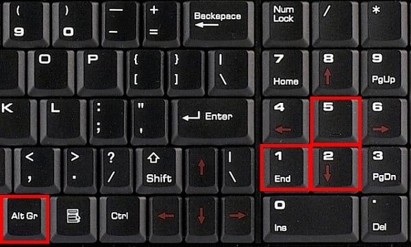
- Нажмите кнопку Num Lock (должен зажечься соответствующий индикатор);
- Нажмите и не отжимайте кнопку Alt;
- Наберите на цифровой клавиатуре справа 251 и отожмите клавишу;
- Вы получите изображение квадратного корня √.

Если вы не знаете, как ввести собаку с клавиатуры, тогда вам обязательно нужно ознакомить с подробной инструкцией по её вводу, так как при наборе E-mail почты без знака собачки не обойтись.
Как использовать таблицу символов
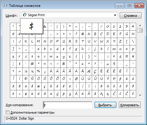
Альтернативой этому варианту является использование специальной таблицы символов, имеющейся в ОС Виндовс, позволяющей использовать корень на клавиатуре. Выполните следующее:
- Нажмите на «Пуск», затем выберите «Все программы»;
- Потом «Стандартные», затем «Служебные», где выберите «Таблица символов».
- Там найдите знак корня √, кликните на него, нажмите на кнопку «Выбрать», затем «Копировать» и скопируйте его в нужный вам текст с помощью клавиш Ctrl+V.
В текстовом редакторе Word (а также в Excel) также имеется соответствующая таблица символов, которую можно использовать для наших задач. Вы можете найти её, перейдя во вкладку «Вставка», и нажав на «Символ» справа, а затем и кликнув на надпись «Другие символы» чуть снизу, это поможет вам в решении вопроса написании корня в Ворде.
Можно, также, использовать опцию «Формула» во вкладке «Вставка» по описанному в данном ролике алгоритму.
Как обозначить степени корня 3,4,5 степени на клавиатуре
Например, корни 3,4,5 степени можно записать так:
X^1/3
X^1/4
X^1/5
Или так:
3√X (вместо числа 3 можете использовать соответствующее обозначение из таблицы символов (³)
4√X
5√X
При этом, несмотря на то, что в системе имеется изображение кубического корня ∛ и четвёртого корня ∜, набрать их через Alt и цифровые клавиши не получится. Это возможно лишь с помощью кодов десятичной системы HTML-код (∛ и ∜) и шестнадцатеричной Юникод (∛ и ∜). По мне, так лучше использовать формы обозначения, описанные мной чуть выше.
Заключение
В данном материале мной были описаны разные варианты написания корня на клавиатуре вашего компьютера. Самые нетерпеливые могут воспользоваться знаком ^, но точнее и правильнее будет, всё же, воспользоваться комбинацией клавиш Alt+251, и поставить знак корня таким, каким он обозначается в соответствии с общепризнанным стандартом символов.

Notation for the (principal) square root of x.

For example, √25 = 5, since 25 = 5 ⋅ 5, or 52 (5 squared).
In mathematics, a square root of a number x is a number y such that y2 = x; in other words, a number y whose square (the result of multiplying the number by itself, or y ⋅ y) is x.[1] For example, 4 and −4 are square roots of 16, because 42 = (−4)2 = 16.
Every nonnegative real number x has a unique nonnegative square root, called the principal square root, which is denoted by  where the symbol
  is called the radical sign[2] or radix. For example, to express the fact that the principal square root of 9 is 3, we write
  . The term (or number) whose square root is being considered is known as the radicand. The radicand is the number or expression underneath the radical sign, in this case 9. For nonnegative x, the principal square root can also be written in exponent notation, as x1/2.
Every positive number x has two square roots: which is positive, and  which is negative. The two roots can be written more concisely using the ± sign as
  . Although the principal square root of a positive number is only one of its two square roots, the designation «the square root» is often used to refer to the principal square root.[3][4]
Square roots of negative numbers can be discussed within the framework of complex numbers. More generally, square roots can be considered in any context in which a notion of the «square» of a mathematical object is defined. These include function spaces and square matrices, among other mathematical structures.
History

The Yale Babylonian Collection YBC 7289 clay tablet was created between 1800 BC and 1600 BC, showing  and
and  respectively as 1;24,51,10 and 0;42,25,35 base 60 numbers on a square crossed by two diagonals.[5] (1;24,51,10) base 60 corresponds to 1.41421296, which is a correct value to 5 decimal points (1.41421356…).
The Rhind Mathematical Papyrus is a copy from 1650 BC of an earlier Berlin Papyrus and other texts – possibly the Kahun Papyrus – that shows how the Egyptians extracted square roots by an inverse proportion method.[6]
In Ancient India, the knowledge of theoretical and applied aspects of square and square root was at least as old as the Sulba Sutras, dated around 800–500 BC (possibly much earlier).[7] A method for finding very good approximations to the square roots of 2 and 3 are given in the Baudhayana Sulba Sutra.[8] Aryabhata, in the Aryabhatiya (section 2.4), has given a method for finding the square root of numbers having many digits.
It was known to the ancient Greeks that square roots of positive integers that are not perfect squares are always irrational numbers: numbers not expressible as a ratio of two integers (that is, they cannot be written exactly as  , where m and n are integers). This is the theorem Euclid X, 9, almost certainly due to Theaetetus dating back to circa 380 BC.[9]
The particular case of the square root of 2 is assumed to date back earlier to the Pythagoreans, and is traditionally attributed to Hippasus.[citation needed] It is exactly the length of the diagonal of a square with side length 1.
In the Chinese mathematical work Writings on Reckoning, written between 202 BC and 186 BC during the early Han Dynasty, the square root is approximated by using an «excess and deficiency» method, which says to «…combine the excess and deficiency as the divisor; (taking) the deficiency numerator multiplied by the excess denominator and the excess numerator times the deficiency denominator, combine them as the dividend.»[10]
A symbol for square roots, written as an elaborate R, was invented by Regiomontanus (1436–1476). An R was also used for radix to indicate square roots in Gerolamo Cardano’s Ars Magna.[11]
According to historian of mathematics D.E. Smith, Aryabhata’s method for finding the square root was first introduced in Europe by Cataneo—in 1546.
According to Jeffrey A. Oaks, Arabs used the letter jīm/ĝīm (ج), the first letter of the word «جذر» (variously transliterated as jaḏr, jiḏr, ǧaḏr or ǧiḏr, «root»), placed in its initial form (ﺟ) over a number to indicate its square root. The letter jīm resembles the present square root shape. Its usage goes as far as the end of the twelfth century in the works of the Moroccan mathematician Ibn al-Yasamin.[12]
The symbol «√» for the square root was first used in print in 1525, in Christoph Rudolff’s Coss.[13]
Properties and uses
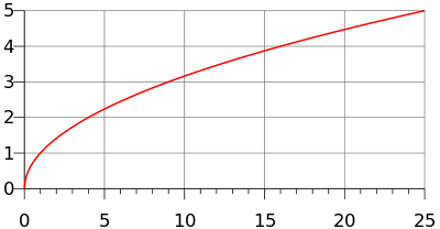
The graph of the function f(x) = √x, made up of half a parabola with a vertical directrix
The principal square root function  (usually just referred to as the «square root function») is a function that maps the set of nonnegative real numbers onto itself. In geometrical terms, the square root function maps the area of a square to its side length.
The square root of x is rational if and only if x is a rational number that can be represented as a ratio of two perfect squares. (See square root of 2 for proofs that this is an irrational number, and quadratic irrational for a proof for all non-square natural numbers.) The square root function maps rational numbers into algebraic numbers, the latter being a superset of the rational numbers).
For all real numbers x,
 (see absolute value)

For all nonnegative real numbers x and y,

and

The square root function is continuous for all nonnegative x, and differentiable for all positive x. If f denotes the square root function, whose derivative is given by:

The Taylor series of  about x = 0 converges for |x| ≤ 1, and is given by

The square root of a nonnegative number is used in the definition of Euclidean norm (and distance), as well as in generalizations such as Hilbert spaces. It defines an important concept of standard deviation used in probability theory and statistics. It has a major use in the formula for roots of a quadratic equation; quadratic fields and rings of quadratic integers, which are based on square roots, are important in algebra and have uses in geometry. Square roots frequently appear in mathematical formulas elsewhere, as well as in many physical laws.
Square roots of positive integers
A positive number has two square roots, one positive, and one negative, which are opposite to each other. When talking of the square root of a positive integer, it is usually the positive square root that is meant.
The square roots of an integer are algebraic integers—more specifically quadratic integers.
The square root of a positive integer is the product of the roots of its prime factors, because the square root of a product is the product of the square roots of the factors. Since  only roots of those primes having an odd power in the factorization are necessary. More precisely, the square root of a prime factorization is

As decimal expansions
The square roots of the perfect squares (e.g., 0, 1, 4, 9, 16) are integers. In all other cases, the square roots of positive integers are irrational numbers, and hence have non-repeating decimals in their decimal representations. Decimal approximations of the square roots of the first few natural numbers are given in the following table.
-
n truncated to 50 decimal places
0 0 1 1 2 1.41421356237309504880168872420969807856967187537694 3 1.73205080756887729352744634150587236694280525381038 4 2 5 2.23606797749978969640917366873127623544061835961152 6 2.44948974278317809819728407470589139196594748065667 7 2.64575131106459059050161575363926042571025918308245 8 2.82842712474619009760337744841939615713934375075389 9 3 10 3.16227766016837933199889354443271853371955513932521

As expansions in other numeral systems
As with before, the square roots of the perfect squares (e.g., 0, 1, 4, 9, 16) are integers. In all other cases, the square roots of positive integers are irrational numbers, and therefore have non-repeating digits in any standard positional notation system.
The square roots of small integers are used in both the SHA-1 and SHA-2 hash function designs to provide nothing up my sleeve numbers.
As periodic continued fractions
One of the most intriguing results from the study of irrational numbers as continued fractions was obtained by Joseph Louis Lagrange c. 1780. Lagrange found that the representation of the square root of any non-square positive integer as a continued fraction is periodic. That is, a certain pattern of partial denominators repeats indefinitely in the continued fraction. In a sense these square roots are the very simplest irrational numbers, because they can be represented with a simple repeating pattern of integers.
-
= [1; 2, 2, …] = [1; 1, 2, 1, 2, …] = [2] = [2; 4, 4, …] = [2; 2, 4, 2, 4, …] = [2; 1, 1, 1, 4, 1, 1, 1, 4, …] = [2; 1, 4, 1, 4, …] = [3] = [3; 6, 6, …] = [3; 3, 6, 3, 6, …] = [3; 2, 6, 2, 6, …] = [3; 1, 1, 1, 1, 6, 1, 1, 1, 1, 6, …] = [3; 1, 2, 1, 6, 1, 2, 1, 6, …] = [3; 1, 6, 1, 6, …] = [4] = [4; 8, 8, …] = [4; 4, 8, 4, 8, …] = [4; 2, 1, 3, 1, 2, 8, 2, 1, 3, 1, 2, 8, …] = [4; 2, 8, 2, 8, …]


The square bracket notation used above is a short form for a continued fraction. Written in the more suggestive algebraic form, the simple continued fraction for the square root of 11, [3; 3, 6, 3, 6, …], looks like this:

where the two-digit pattern {3, 6} repeats over and over again in the partial denominators. Since 11 = 32 + 2, the above is also identical to the following generalized continued fractions:

Computation
Square roots of positive numbers are not in general rational numbers, and so cannot be written as a terminating or recurring decimal expression. Therefore in general any attempt to compute a square root expressed in decimal form can only yield an approximation, though a sequence of increasingly accurate approximations can be obtained.
Most pocket calculators have a square root key. Computer spreadsheets and other software are also frequently used to calculate square roots. Pocket calculators typically implement efficient routines, such as the Newton’s method (frequently with an initial guess of 1), to compute the square root of a positive real number.[14][15] When computing square roots with logarithm tables or slide rules, one can exploit the identities

where ln and log10 are the natural and base-10 logarithms.
By trial-and-error,[16] one can square an estimate for  and raise or lower the estimate until it agrees to sufficient accuracy. For this technique it is prudent to use the identity

as it allows one to adjust the estimate x by some amount c and measure the square of the adjustment in terms of the original estimate and its square. Furthermore, (x + c)2 ≈ x2 + 2xc when c is close to 0, because the tangent line to the graph of x2 + 2xc + c2 at c = 0, as a function of c alone, is y = 2xc + x2. Thus, small adjustments to x can be planned out by setting 2xc to a, or c = a/(2x).
The most common iterative method of square root calculation by hand is known as the «Babylonian method» or «Heron’s method» after the first-century Greek philosopher Heron of Alexandria, who first described it.[17]
The method uses the same iterative scheme as the Newton–Raphson method yields when applied to the function y = f(x) = x2 − a, using the fact that its slope at any point is dy/dx = f′(x) = 2x, but predates it by many centuries.[18]
The algorithm is to repeat a simple calculation that results in a number closer to the actual square root each time it is repeated with its result as the new input. The motivation is that if x is an overestimate to the square root of a nonnegative real number a then a/x will be an underestimate and so the average of these two numbers is a better approximation than either of them. However, the inequality of arithmetic and geometric means shows this average is always an overestimate of the square root (as noted below), and so it can serve as a new overestimate with which to repeat the process, which converges as a consequence of the successive overestimates and underestimates being closer to each other after each iteration. To find x:
- Start with an arbitrary positive start value x. The closer to the square root of a, the fewer the iterations that will be needed to achieve the desired precision.
- Replace x by the average (x + a/x) / 2 between x and a/x.
- Repeat from step 2, using this average as the new value of x.
That is, if an arbitrary guess for is x0, and xn + 1 = (xn + a/xn) / 2, then each xn is an approximation of which is better for large n than for small n. If a is positive, the convergence is quadratic, which means that in approaching the limit, the number of correct digits roughly doubles in each next iteration. If a = 0, the convergence is only linear.
Using the identity

the computation of the square root of a positive number can be reduced to that of a number in the range [1,4). This simplifies finding a start value for the iterative method that is close to the square root, for which a polynomial or piecewise-linear approximation can be used.
The time complexity for computing a square root with n digits of precision is equivalent to that of multiplying two n-digit numbers.
Another useful method for calculating the square root is the shifting nth root algorithm, applied for n = 2.
The name of the square root function varies from programming language to programming language, with sqrt[19] (often pronounced «squirt» [20]) being common, used in C, C++, and derived languages like JavaScript, PHP, and Python.
Square roots of negative and complex numbers

First leaf of the complex square root
Second leaf of the complex square root

Using the Riemann surface of the square root, it is shown how the two leaves fit together
The square of any positive or negative number is positive, and the square of 0 is 0. Therefore, no negative number can have a real square root. However, it is possible to work with a more inclusive set of numbers, called the complex numbers, that does contain solutions to the square root of a negative number. This is done by introducing a new number, denoted by i (sometimes by j, especially in the context of electricity where «i» traditionally represents electric current) and called the imaginary unit, which is defined such that i2 = −1. Using this notation, we can think of i as the square root of −1, but we also have (−i)2 = i2 = −1 and so −i is also a square root of −1. By convention, the principal square root of −1 is i, or more generally, if x is any nonnegative number, then the principal square root of −x is

The right side (as well as its negative) is indeed a square root of −x, since

For every non-zero complex number z there exist precisely two numbers w such that w2 = z: the principal square root of z (defined below), and its negative.
Principal square root of a complex number

Geometric representation of the 2nd to 6th roots of a complex number z, in polar form reiφ where r = |z | and φ = arg z. If z is real, φ = 0 or π. Principal roots are shown in black.
To find a definition for the square root that allows us to consistently choose a single value, called the principal value, we start by observing that any complex number  can be viewed as a point in the plane,
  expressed using Cartesian coordinates. The same point may be reinterpreted using polar coordinates as the pair
  where
where  is the distance of the point from the origin, and
  is the angle that the line from the origin to the point makes with the positive real (
 ) axis. In complex analysis, the location of this point is conventionally written
  If
If

then the principal square root of  is defined to be the following:

The principal square root function is thus defined using the nonpositive real axis as a branch cut.
If is a non-negative real number (which happens if and only if  ) then the principal square root of is
  in other words, the principal square root of a non-negative real number is just the usual non-negative square root.
It is important that  because if, for example,
  (so
(so  ) then the principal square root is

but using  would instead produce the other square root
The principal square root function is holomorphic everywhere except on the set of non-positive real numbers (on strictly negative reals it is not even continuous). The above Taylor series for remains valid for complex numbers with 
The above can also be expressed in terms of trigonometric functions:

Algebraic formula

When the number is expressed using its real and imaginary parts, the following formula can be used for the principal square root:[21][22]

where sgn(y) is the sign of y (except that, here, sgn(0) = 1). In particular, the imaginary parts of the original number and the principal value of its square root have the same sign. The real part of the principal value of the square root is always nonnegative.
For example, the principal square roots of ±i are given by:

Notes
In the following, the complex z and w may be expressed as:
where  and
and  .
.
Because of the discontinuous nature of the square root function in the complex plane, the following laws are not true in general.
A similar problem appears with other complex functions with branch cuts, e.g., the complex logarithm and the relations logz + logw = log(zw) or log(z*) = log(z)* which are not true in general.
Wrongly assuming one of these laws underlies several faulty «proofs», for instance the following one showing that −1 = 1:

The third equality cannot be justified (see invalid proof).[23]: Chapter VI Some fallacies in algebra and trigonometry, Section I The fallacies, Subsection 2 The fallacy that +1 = -1 It can be made to hold by changing the meaning of √ so that this no longer represents the principal square root (see above) but selects a branch for the square root that contains  The left-hand side becomes either

if the branch includes +i or

if the branch includes −i, while the right-hand side becomes

where the last equality,  is a consequence of the choice of branch in the redefinition of √.
Nth roots and polynomial roots
The definition of a square root of as a number  such that
  has been generalized in the following way.
A cube root of is a number such that  ; it is denoted
 ![{displaystyle {sqrt[{3}]{x}}.}](https://wikimedia.org/api/rest_v1/media/math/render/svg/d19f445fd1e8ab7046f090279ee7cf3506f0cf50)
If n is an integer greater than two, a nth root of is a number such that  ; it is denoted
 ![{displaystyle {sqrt[{n}]{x}}.}](https://wikimedia.org/api/rest_v1/media/math/render/svg/8562e64a6bc6e408ddf67f055682c4dc9c9f957f)
Given any polynomial p, a root of p is a number y such that p(y) = 0. For example, the nth roots of x are the roots of the polynomial (in y) 
Abel–Ruffini theorem states that, in general, the roots of a polynomial of degree five or higher cannot be expressed in terms of nth roots.
Square roots of matrices and operators
If A is a positive-definite matrix or operator, then there exists precisely one positive definite matrix or operator B with B2 = A; we then define A1/2 = B. In general matrices may have multiple square roots or even an infinitude of them. For example, the 2 × 2 identity matrix has an infinity of square roots,[24] though only one of them is positive definite.
In integral domains, including fields
Each element of an integral domain has no more than 2 square roots. The difference of two squares identity u2 − v2 = (u − v)(u + v) is proved using the commutativity of multiplication. If u and v are square roots of the same element, then u2 − v2 = 0. Because there are no zero divisors this implies u = v or u + v = 0, where the latter means that two roots are additive inverses of each other. In other words if an element a square root u of an element a exists, then the only square roots of a are u and −u. The only square root of 0 in an integral domain is 0 itself.
In a field of characteristic 2, an element either has one square root or does not have any at all, because each element is its own additive inverse, so that −u = u. If the field is finite of characteristic 2 then every element has a unique square root. In a field of any other characteristic, any non-zero element either has two square roots, as explained above, or does not have any.
Given an odd prime number p, let q = pe for some positive integer e. A non-zero element of the field Fq with q elements is a quadratic residue if it has a square root in Fq. Otherwise, it is a quadratic non-residue. There are (q − 1)/2 quadratic residues and (q − 1)/2 quadratic non-residues; zero is not counted in either class. The quadratic residues form a group under multiplication. The properties of quadratic residues are widely used in number theory.
In rings in general
Unlike in an integral domain, a square root in an arbitrary (unital) ring need not be unique up to sign. For example, in the ring  of integers modulo 8 (which is commutative, but has zero divisors), the element 1 has four distinct square roots: ±1 and ±3.
Another example is provided by the ring of quaternions  which has no zero divisors, but is not commutative. Here, the element −1 has infinitely many square roots, including ±i, ±j, and ±k. In fact, the set of square roots of −1 is exactly

A square root of 0 is either 0 or a zero divisor. Thus in rings where zero divisors do not exist, it is uniquely 0. However, rings with zero divisors may have multiple square roots of 0. For example, in  any multiple of n is a square root of 0.
Geometric construction of the square root


The square root of a positive number is usually defined as the side length of a square with the area equal to the given number. But the square shape is not necessary for it: if one of two similar planar Euclidean objects has the area a times greater than another, then the ratio of their linear sizes is .
A square root can be constructed with a compass and straightedge. In his Elements, Euclid (fl. 300 BC) gave the construction of the geometric mean of two quantities in two different places: Proposition II.14 and Proposition VI.13. Since the geometric mean of a and b is  , one can construct simply by taking b = 1.
The construction is also given by Descartes in his La Géométrie, see figure 2 on page 2. However, Descartes made no claim to originality and his audience would have been quite familiar with Euclid.
Euclid’s second proof in Book VI depends on the theory of similar triangles. Let AHB be a line segment of length a + b with AH = a and HB = b. Construct the circle with AB as diameter and let C be one of the two intersections of the perpendicular chord at H with the circle and denote the length CH as h. Then, using Thales’ theorem and, as in the proof of Pythagoras’ theorem by similar triangles, triangle AHC is similar to triangle CHB (as indeed both are to triangle ACB, though we don’t need that, but it is the essence of the proof of Pythagoras’ theorem) so that AH:CH is as HC:HB, i.e. a/h = h/b, from which we conclude by cross-multiplication that h2 = ab, and finally that  . When marking the midpoint O of the line segment AB and drawing the radius OC of length (a + b)/2, then clearly OC > CH, i.e.
  (with equality if and only if a = b), which is the arithmetic–geometric mean inequality for two variables and, as noted above, is the basis of the Ancient Greek understanding of «Heron’s method».
Another method of geometric construction uses right triangles and induction:  can be constructed, and once
  has been constructed, the right triangle with legs 1 and has a hypotenuse of
  . Constructing successive square roots in this manner yields the Spiral of Theodorus depicted above.
See also
- Apotome (mathematics)
- Cube root
- Functional square root
- Integer square root
- Nested radical
- Nth root
- Root of unity
- Solving quadratic equations with continued fractions
- Square root principle
- Quantum gate § Square root of NOT gate (√NOT)
Notes
- ^ Gel’fand, p. 120 Archived 2016-09-02 at the Wayback Machine
- ^ «Squares and Square Roots». www.mathsisfun.com. Retrieved 2020-08-28.
- ^ Zill, Dennis G.; Shanahan, Patrick (2008). A First Course in Complex Analysis With Applications (2nd ed.). Jones & Bartlett Learning. p. 78. ISBN 978-0-7637-5772-4. Archived from the original on 2016-09-01. Extract of page 78 Archived 2016-09-01 at the Wayback Machine
- ^ Weisstein, Eric W. «Square Root». mathworld.wolfram.com. Retrieved 2020-08-28.
- ^ «Analysis of YBC 7289». ubc.ca. Retrieved 19 January 2015.
- ^ Anglin, W.S. (1994). Mathematics: A Concise History and Philosophy. New York: Springer-Verlag.
- ^ Seidenberg, A. (1961). «The ritual origin of geometry». Archive for History of Exact Sciences. 1 (5): 488–527. doi:10.1007/bf00327767. ISSN 0003-9519.
Seidenberg (pp. 501-505) proposes: «It is the distinction between use and origin.» [By analogy] «KEPLER needed the ellipse to describe the paths of the planets around the sun; he did not, however invent the ellipse, but made use of a curve that had been lying around for nearly 2000 years». In this manner Seidenberg argues: «Although the date of a manuscript or text cannot give us the age of the practices it discloses, nonetheless the evidence is contained in manuscripts.» Seidenberg quotes Thibaut from 1875: «Regarding the time in which the Sulvasutras may have been composed, it is impossible to give more accurate information than we are able to give about the date of the Kalpasutras. But whatever the period may have been during which Kalpasutras and Sulvasutras were composed in the form now before us, we must keep in view that they only give a systematically arranged description of sacrificial rites, which had been practiced during long preceding ages.» Lastly, Seidenberg summarizes: «In 1899, THIBAUT ventured to assign the fourth or the third centuries B.C. as the latest possible date for the composition of the Sulvasutras (it being understood that this refers to a codification of far older material).»
- ^ Joseph, ch.8.
- ^ Heath, Sir Thomas L. (1908). The Thirteen Books of The Elements, Vol. 3. Cambridge University Press. p. 3.
- ^ Dauben (2007), p. 210.
- ^ «The Development of Algebra — 2». maths.org. Archived from the original on 24 November 2014. Retrieved 19 January 2015.
- ^ * Oaks, Jeffrey A. (2012). Algebraic Symbolism in Medieval Arabic Algebra (PDF) (Thesis). Philosophica. p. 36. Archived (PDF) from the original on 2016-12-03.
- ^ Manguel, Alberto (2006). «Done on paper: the dual nature of numbers and the page». The Life of Numbers. ISBN 84-86882-14-1.
- ^ Parkhurst, David F. (2006). Introduction to Applied Mathematics for Environmental Science. Springer. pp. 241. ISBN 9780387342283.
- ^ Solow, Anita E. (1993). Learning by Discovery: A Lab Manual for Calculus. Cambridge University Press. pp. 48. ISBN 9780883850831.
- ^ Aitken, Mike; Broadhurst, Bill; Hladky, Stephen (2009). Mathematics for Biological Scientists. Garland Science. p. 41. ISBN 978-1-136-84393-8. Archived from the original on 2017-03-01. Extract of page 41 Archived 2017-03-01 at the Wayback Machine
- ^ Heath, Sir Thomas L. (1921). A History of Greek Mathematics, Vol. 2. Oxford: Clarendon Press. pp. 323–324.
- ^ Muller, Jean-Mic (2006). Elementary functions: algorithms and implementation. Springer. pp. 92–93. ISBN 0-8176-4372-9., Chapter 5, p 92 Archived 2016-09-01 at the Wayback Machine
- ^ «Function sqrt». CPlusPlus.com. The C++ Resources Network. 2016. Archived from the original on November 22, 2012. Retrieved June 24, 2016.
- ^ Overland, Brian (2013). C++ for the Impatient. Addison-Wesley. p. 338. ISBN 9780133257120. OCLC 850705706. Archived from the original on September 1, 2016. Retrieved June 24, 2016.
- ^ Abramowitz, Milton; Stegun, Irene A. (1964). Handbook of mathematical functions with formulas, graphs, and mathematical tables. Courier Dover Publications. p. 17. ISBN 0-486-61272-4. Archived from the original on 2016-04-23., Section 3.7.27, p. 17 Archived 2009-09-10 at the Wayback Machine
- ^ Cooke, Roger (2008). Classical algebra: its nature, origins, and uses. John Wiley and Sons. p. 59. ISBN 978-0-470-25952-8. Archived from the original on 2016-04-23.
- ^ Maxwell, E. A. (1959). Fallacies in Mathematics. Cambridge University Press.
- ^ Mitchell, Douglas W., «Using Pythagorean triples to generate square roots of I2«, Mathematical Gazette 87, November 2003, 499–500.
References
- Dauben, Joseph W. (2007). «Chinese Mathematics I». In Katz, Victor J. (ed.). The Mathematics of Egypt, Mesopotamia, China, India, and Islam. Princeton: Princeton University Press. ISBN 978-0-691-11485-9.
- Gel’fand, Izrael M.; Shen, Alexander (1993). Algebra (3rd ed.). Birkhäuser. p. 120. ISBN 0-8176-3677-3.
- Joseph, George (2000). The Crest of the Peacock. Princeton: Princeton University Press. ISBN 0-691-00659-8.
- Smith, David (1958). History of Mathematics. Vol. 2. New York: Dover Publications. ISBN 978-0-486-20430-7.
- Selin, Helaine (2008), Encyclopaedia of the History of Science, Technology, and Medicine in Non-Western Cultures, Springer, Bibcode:2008ehst.book…..S, ISBN 978-1-4020-4559-2.
External links
- Algorithms, implementations, and more – Paul Hsieh’s square roots webpage
- How to manually find a square root
- AMS Featured Column, Galileo’s Arithmetic by Tony Philips – includes a section on how Galileo found square roots
Notation for the (principal) square root of x.
For example, √25 = 5, since 25 = 5 ⋅ 5, or 52 (5 squared).
In mathematics, a square root of a number x is a number y such that y2 = x; in other words, a number y whose square (the result of multiplying the number by itself, or y ⋅ y) is x.[1] For example, 4 and −4 are square roots of 16, because 42 = (−4)2 = 16.
Every nonnegative real number x has a unique nonnegative square root, called the principal square root, which is denoted by where the symbol is called the radical sign[2] or radix. For example, to express the fact that the principal square root of 9 is 3, we write . The term (or number) whose square root is being considered is known as the radicand. The radicand is the number or expression underneath the radical sign, in this case 9. For nonnegative x, the principal square root can also be written in exponent notation, as x1/2.
Every positive number x has two square roots: which is positive, and which is negative. The two roots can be written more concisely using the ± sign as . Although the principal square root of a positive number is only one of its two square roots, the designation «the square root» is often used to refer to the principal square root.[3][4]
Square roots of negative numbers can be discussed within the framework of complex numbers. More generally, square roots can be considered in any context in which a notion of the «square» of a mathematical object is defined. These include function spaces and square matrices, among other mathematical structures.
History
The Yale Babylonian Collection YBC 7289 clay tablet was created between 1800 BC and 1600 BC, showing and respectively as 1;24,51,10 and 0;42,25,35 base 60 numbers on a square crossed by two diagonals.[5] (1;24,51,10) base 60 corresponds to 1.41421296, which is a correct value to 5 decimal points (1.41421356…).
The Rhind Mathematical Papyrus is a copy from 1650 BC of an earlier Berlin Papyrus and other texts – possibly the Kahun Papyrus – that shows how the Egyptians extracted square roots by an inverse proportion method.[6]
In Ancient India, the knowledge of theoretical and applied aspects of square and square root was at least as old as the Sulba Sutras, dated around 800–500 BC (possibly much earlier).[7] A method for finding very good approximations to the square roots of 2 and 3 are given in the Baudhayana Sulba Sutra.[8] Aryabhata, in the Aryabhatiya (section 2.4), has given a method for finding the square root of numbers having many digits.
It was known to the ancient Greeks that square roots of positive integers that are not perfect squares are always irrational numbers: numbers not expressible as a ratio of two integers (that is, they cannot be written exactly as , where m and n are integers). This is the theorem Euclid X, 9, almost certainly due to Theaetetus dating back to circa 380 BC.[9]
The particular case of the square root of 2 is assumed to date back earlier to the Pythagoreans, and is traditionally attributed to Hippasus.[citation needed] It is exactly the length of the diagonal of a square with side length 1.
In the Chinese mathematical work Writings on Reckoning, written between 202 BC and 186 BC during the early Han Dynasty, the square root is approximated by using an «excess and deficiency» method, which says to «…combine the excess and deficiency as the divisor; (taking) the deficiency numerator multiplied by the excess denominator and the excess numerator times the deficiency denominator, combine them as the dividend.»[10]
A symbol for square roots, written as an elaborate R, was invented by Regiomontanus (1436–1476). An R was also used for radix to indicate square roots in Gerolamo Cardano’s Ars Magna.[11]
According to historian of mathematics D.E. Smith, Aryabhata’s method for finding the square root was first introduced in Europe by Cataneo—in 1546.
According to Jeffrey A. Oaks, Arabs used the letter jīm/ĝīm (ج), the first letter of the word «جذر» (variously transliterated as jaḏr, jiḏr, ǧaḏr or ǧiḏr, «root»), placed in its initial form (ﺟ) over a number to indicate its square root. The letter jīm resembles the present square root shape. Its usage goes as far as the end of the twelfth century in the works of the Moroccan mathematician Ibn al-Yasamin.[12]
The symbol «√» for the square root was first used in print in 1525, in Christoph Rudolff’s Coss.[13]
Properties and uses
The graph of the function f(x) = √x, made up of half a parabola with a vertical directrix
The principal square root function (usually just referred to as the «square root function») is a function that maps the set of nonnegative real numbers onto itself. In geometrical terms, the square root function maps the area of a square to its side length.
The square root of x is rational if and only if x is a rational number that can be represented as a ratio of two perfect squares. (See square root of 2 for proofs that this is an irrational number, and quadratic irrational for a proof for all non-square natural numbers.) The square root function maps rational numbers into algebraic numbers, the latter being a superset of the rational numbers).
For all real numbers x,
- (see absolute value)
For all nonnegative real numbers x and y,
and
The square root function is continuous for all nonnegative x, and differentiable for all positive x. If f denotes the square root function, whose derivative is given by:
The Taylor series of about x = 0 converges for |x| ≤ 1, and is given by
The square root of a nonnegative number is used in the definition of Euclidean norm (and distance), as well as in generalizations such as Hilbert spaces. It defines an important concept of standard deviation used in probability theory and statistics. It has a major use in the formula for roots of a quadratic equation; quadratic fields and rings of quadratic integers, which are based on square roots, are important in algebra and have uses in geometry. Square roots frequently appear in mathematical formulas elsewhere, as well as in many physical laws.
Square roots of positive integers
A positive number has two square roots, one positive, and one negative, which are opposite to each other. When talking of the square root of a positive integer, it is usually the positive square root that is meant.
The square roots of an integer are algebraic integers—more specifically quadratic integers.
The square root of a positive integer is the product of the roots of its prime factors, because the square root of a product is the product of the square roots of the factors. Since only roots of those primes having an odd power in the factorization are necessary. More precisely, the square root of a prime factorization is
As decimal expansions
The square roots of the perfect squares (e.g., 0, 1, 4, 9, 16) are integers. In all other cases, the square roots of positive integers are irrational numbers, and hence have non-repeating decimals in their decimal representations. Decimal approximations of the square roots of the first few natural numbers are given in the following table.
-
n truncated to 50 decimal places
0 0 1 1 2 1.41421356237309504880168872420969807856967187537694 3 1.73205080756887729352744634150587236694280525381038 4 2 5 2.23606797749978969640917366873127623544061835961152 6 2.44948974278317809819728407470589139196594748065667 7 2.64575131106459059050161575363926042571025918308245 8 2.82842712474619009760337744841939615713934375075389 9 3 10 3.16227766016837933199889354443271853371955513932521
As expansions in other numeral systems
As with before, the square roots of the perfect squares (e.g., 0, 1, 4, 9, 16) are integers. In all other cases, the square roots of positive integers are irrational numbers, and therefore have non-repeating digits in any standard positional notation system.
The square roots of small integers are used in both the SHA-1 and SHA-2 hash function designs to provide nothing up my sleeve numbers.
As periodic continued fractions
One of the most intriguing results from the study of irrational numbers as continued fractions was obtained by Joseph Louis Lagrange c. 1780. Lagrange found that the representation of the square root of any non-square positive integer as a continued fraction is periodic. That is, a certain pattern of partial denominators repeats indefinitely in the continued fraction. In a sense these square roots are the very simplest irrational numbers, because they can be represented with a simple repeating pattern of integers.
-
= [1; 2, 2, …] = [1; 1, 2, 1, 2, …] = [2] = [2; 4, 4, …] = [2; 2, 4, 2, 4, …] = [2; 1, 1, 1, 4, 1, 1, 1, 4, …] = [2; 1, 4, 1, 4, …] = [3] = [3; 6, 6, …] = [3; 3, 6, 3, 6, …] = [3; 2, 6, 2, 6, …] = [3; 1, 1, 1, 1, 6, 1, 1, 1, 1, 6, …] = [3; 1, 2, 1, 6, 1, 2, 1, 6, …] = [3; 1, 6, 1, 6, …] = [4] = [4; 8, 8, …] = [4; 4, 8, 4, 8, …] = [4; 2, 1, 3, 1, 2, 8, 2, 1, 3, 1, 2, 8, …] = [4; 2, 8, 2, 8, …]
The square bracket notation used above is a short form for a continued fraction. Written in the more suggestive algebraic form, the simple continued fraction for the square root of 11, [3; 3, 6, 3, 6, …], looks like this:
where the two-digit pattern {3, 6} repeats over and over again in the partial denominators. Since 11 = 32 + 2, the above is also identical to the following generalized continued fractions:
Computation
Square roots of positive numbers are not in general rational numbers, and so cannot be written as a terminating or recurring decimal expression. Therefore in general any attempt to compute a square root expressed in decimal form can only yield an approximation, though a sequence of increasingly accurate approximations can be obtained.
Most pocket calculators have a square root key. Computer spreadsheets and other software are also frequently used to calculate square roots. Pocket calculators typically implement efficient routines, such as the Newton’s method (frequently with an initial guess of 1), to compute the square root of a positive real number.[14][15] When computing square roots with logarithm tables or slide rules, one can exploit the identities
where ln and log10 are the natural and base-10 logarithms.
By trial-and-error,[16] one can square an estimate for and raise or lower the estimate until it agrees to sufficient accuracy. For this technique it is prudent to use the identity
as it allows one to adjust the estimate x by some amount c and measure the square of the adjustment in terms of the original estimate and its square. Furthermore, (x + c)2 ≈ x2 + 2xc when c is close to 0, because the tangent line to the graph of x2 + 2xc + c2 at c = 0, as a function of c alone, is y = 2xc + x2. Thus, small adjustments to x can be planned out by setting 2xc to a, or c = a/(2x).
The most common iterative method of square root calculation by hand is known as the «Babylonian method» or «Heron’s method» after the first-century Greek philosopher Heron of Alexandria, who first described it.[17]
The method uses the same iterative scheme as the Newton–Raphson method yields when applied to the function y = f(x) = x2 − a, using the fact that its slope at any point is dy/dx = f′(x) = 2x, but predates it by many centuries.[18]
The algorithm is to repeat a simple calculation that results in a number closer to the actual square root each time it is repeated with its result as the new input. The motivation is that if x is an overestimate to the square root of a nonnegative real number a then a/x will be an underestimate and so the average of these two numbers is a better approximation than either of them. However, the inequality of arithmetic and geometric means shows this average is always an overestimate of the square root (as noted below), and so it can serve as a new overestimate with which to repeat the process, which converges as a consequence of the successive overestimates and underestimates being closer to each other after each iteration. To find x:
- Start with an arbitrary positive start value x. The closer to the square root of a, the fewer the iterations that will be needed to achieve the desired precision.
- Replace x by the average (x + a/x) / 2 between x and a/x.
- Repeat from step 2, using this average as the new value of x.
That is, if an arbitrary guess for is x0, and xn + 1 = (xn + a/xn) / 2, then each xn is an approximation of which is better for large n than for small n. If a is positive, the convergence is quadratic, which means that in approaching the limit, the number of correct digits roughly doubles in each next iteration. If a = 0, the convergence is only linear.
Using the identity
the computation of the square root of a positive number can be reduced to that of a number in the range [1,4). This simplifies finding a start value for the iterative method that is close to the square root, for which a polynomial or piecewise-linear approximation can be used.
The time complexity for computing a square root with n digits of precision is equivalent to that of multiplying two n-digit numbers.
Another useful method for calculating the square root is the shifting nth root algorithm, applied for n = 2.
The name of the square root function varies from programming language to programming language, with sqrt[19] (often pronounced «squirt» [20]) being common, used in C, C++, and derived languages like JavaScript, PHP, and Python.
Square roots of negative and complex numbers
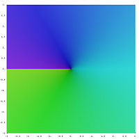
First leaf of the complex square root
Second leaf of the complex square root
Using the Riemann surface of the square root, it is shown how the two leaves fit together
The square of any positive or negative number is positive, and the square of 0 is 0. Therefore, no negative number can have a real square root. However, it is possible to work with a more inclusive set of numbers, called the complex numbers, that does contain solutions to the square root of a negative number. This is done by introducing a new number, denoted by i (sometimes by j, especially in the context of electricity where «i» traditionally represents electric current) and called the imaginary unit, which is defined such that i2 = −1. Using this notation, we can think of i as the square root of −1, but we also have (−i)2 = i2 = −1 and so −i is also a square root of −1. By convention, the principal square root of −1 is i, or more generally, if x is any nonnegative number, then the principal square root of −x is
The right side (as well as its negative) is indeed a square root of −x, since
For every non-zero complex number z there exist precisely two numbers w such that w2 = z: the principal square root of z (defined below), and its negative.
Principal square root of a complex number
Geometric representation of the 2nd to 6th roots of a complex number z, in polar form reiφ where r = |z | and φ = arg z. If z is real, φ = 0 or π. Principal roots are shown in black.
To find a definition for the square root that allows us to consistently choose a single value, called the principal value, we start by observing that any complex number can be viewed as a point in the plane, expressed using Cartesian coordinates. The same point may be reinterpreted using polar coordinates as the pair where is the distance of the point from the origin, and is the angle that the line from the origin to the point makes with the positive real () axis. In complex analysis, the location of this point is conventionally written If
then the principal square root of is defined to be the following:
The principal square root function is thus defined using the nonpositive real axis as a branch cut.
If is a non-negative real number (which happens if and only if ) then the principal square root of is in other words, the principal square root of a non-negative real number is just the usual non-negative square root.
It is important that because if, for example, (so ) then the principal square root is
but using would instead produce the other square root
The principal square root function is holomorphic everywhere except on the set of non-positive real numbers (on strictly negative reals it is not even continuous). The above Taylor series for remains valid for complex numbers with
The above can also be expressed in terms of trigonometric functions:
Algebraic formula
When the number is expressed using its real and imaginary parts, the following formula can be used for the principal square root:[21][22]
where sgn(y) is the sign of y (except that, here, sgn(0) = 1). In particular, the imaginary parts of the original number and the principal value of its square root have the same sign. The real part of the principal value of the square root is always nonnegative.
For example, the principal square roots of ±i are given by:
Notes
In the following, the complex z and w may be expressed as:
where and .
Because of the discontinuous nature of the square root function in the complex plane, the following laws are not true in general.
A similar problem appears with other complex functions with branch cuts, e.g., the complex logarithm and the relations logz + logw = log(zw) or log(z*) = log(z)* which are not true in general.
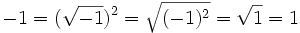
Wrongly assuming one of these laws underlies several faulty «proofs», for instance the following one showing that −1 = 1:
The third equality cannot be justified (see invalid proof).[23]: Chapter VI Some fallacies in algebra and trigonometry, Section I The fallacies, Subsection 2 The fallacy that +1 = -1 It can be made to hold by changing the meaning of √ so that this no longer represents the principal square root (see above) but selects a branch for the square root that contains The left-hand side becomes either
if the branch includes +i or
if the branch includes −i, while the right-hand side becomes
where the last equality, is a consequence of the choice of branch in the redefinition of √.
Nth roots and polynomial roots
The definition of a square root of as a number such that has been generalized in the following way.
A cube root of is a number such that ; it is denoted
If n is an integer greater than two, a nth root of is a number such that ; it is denoted
Given any polynomial p, a root of p is a number y such that p(y) = 0. For example, the nth roots of x are the roots of the polynomial (in y)
Abel–Ruffini theorem states that, in general, the roots of a polynomial of degree five or higher cannot be expressed in terms of nth roots.
Square roots of matrices and operators
If A is a positive-definite matrix or operator, then there exists precisely one positive definite matrix or operator B with B2 = A; we then define A1/2 = B. In general matrices may have multiple square roots or even an infinitude of them. For example, the 2 × 2 identity matrix has an infinity of square roots,[24] though only one of them is positive definite.
In integral domains, including fields
Each element of an integral domain has no more than 2 square roots. The difference of two squares identity u2 − v2 = (u − v)(u + v) is proved using the commutativity of multiplication. If u and v are square roots of the same element, then u2 − v2 = 0. Because there are no zero divisors this implies u = v or u + v = 0, where the latter means that two roots are additive inverses of each other. In other words if an element a square root u of an element a exists, then the only square roots of a are u and −u. The only square root of 0 in an integral domain is 0 itself.
In a field of characteristic 2, an element either has one square root or does not have any at all, because each element is its own additive inverse, so that −u = u. If the field is finite of characteristic 2 then every element has a unique square root. In a field of any other characteristic, any non-zero element either has two square roots, as explained above, or does not have any.
Given an odd prime number p, let q = pe for some positive integer e. A non-zero element of the field Fq with q elements is a quadratic residue if it has a square root in Fq. Otherwise, it is a quadratic non-residue. There are (q − 1)/2 quadratic residues and (q − 1)/2 quadratic non-residues; zero is not counted in either class. The quadratic residues form a group under multiplication. The properties of quadratic residues are widely used in number theory.
In rings in general
Unlike in an integral domain, a square root in an arbitrary (unital) ring need not be unique up to sign. For example, in the ring of integers modulo 8 (which is commutative, but has zero divisors), the element 1 has four distinct square roots: ±1 and ±3.
Another example is provided by the ring of quaternions which has no zero divisors, but is not commutative. Here, the element −1 has infinitely many square roots, including ±i, ±j, and ±k. In fact, the set of square roots of −1 is exactly
A square root of 0 is either 0 or a zero divisor. Thus in rings where zero divisors do not exist, it is uniquely 0. However, rings with zero divisors may have multiple square roots of 0. For example, in any multiple of n is a square root of 0.
Geometric construction of the square root
The square root of a positive number is usually defined as the side length of a square with the area equal to the given number. But the square shape is not necessary for it: if one of two similar planar Euclidean objects has the area a times greater than another, then the ratio of their linear sizes is .
A square root can be constructed with a compass and straightedge. In his Elements, Euclid (fl. 300 BC) gave the construction of the geometric mean of two quantities in two different places: Proposition II.14 and Proposition VI.13. Since the geometric mean of a and b is , one can construct simply by taking b = 1.
The construction is also given by Descartes in his La Géométrie, see figure 2 on page 2. However, Descartes made no claim to originality and his audience would have been quite familiar with Euclid.
Euclid’s second proof in Book VI depends on the theory of similar triangles. Let AHB be a line segment of length a + b with AH = a and HB = b. Construct the circle with AB as diameter and let C be one of the two intersections of the perpendicular chord at H with the circle and denote the length CH as h. Then, using Thales’ theorem and, as in the proof of Pythagoras’ theorem by similar triangles, triangle AHC is similar to triangle CHB (as indeed both are to triangle ACB, though we don’t need that, but it is the essence of the proof of Pythagoras’ theorem) so that AH:CH is as HC:HB, i.e. a/h = h/b, from which we conclude by cross-multiplication that h2 = ab, and finally that . When marking the midpoint O of the line segment AB and drawing the radius OC of length (a + b)/2, then clearly OC > CH, i.e. (with equality if and only if a = b), which is the arithmetic–geometric mean inequality for two variables and, as noted above, is the basis of the Ancient Greek understanding of «Heron’s method».
Another method of geometric construction uses right triangles and induction: can be constructed, and once has been constructed, the right triangle with legs 1 and has a hypotenuse of . Constructing successive square roots in this manner yields the Spiral of Theodorus depicted above.
See also
- Apotome (mathematics)
- Cube root
- Functional square root
- Integer square root
- Nested radical
- Nth root
- Root of unity
- Solving quadratic equations with continued fractions
- Square root principle
- Quantum gate § Square root of NOT gate (√NOT)
Notes
- ^ Gel’fand, p. 120 Archived 2016-09-02 at the Wayback Machine
- ^ «Squares and Square Roots». www.mathsisfun.com. Retrieved 2020-08-28.
- ^ Zill, Dennis G.; Shanahan, Patrick (2008). A First Course in Complex Analysis With Applications (2nd ed.). Jones & Bartlett Learning. p. 78. ISBN 978-0-7637-5772-4. Archived from the original on 2016-09-01. Extract of page 78 Archived 2016-09-01 at the Wayback Machine
- ^ Weisstein, Eric W. «Square Root». mathworld.wolfram.com. Retrieved 2020-08-28.
- ^ «Analysis of YBC 7289». ubc.ca. Retrieved 19 January 2015.
- ^ Anglin, W.S. (1994). Mathematics: A Concise History and Philosophy. New York: Springer-Verlag.
- ^ Seidenberg, A. (1961). «The ritual origin of geometry». Archive for History of Exact Sciences. 1 (5): 488–527. doi:10.1007/bf00327767. ISSN 0003-9519.
Seidenberg (pp. 501-505) proposes: «It is the distinction between use and origin.» [By analogy] «KEPLER needed the ellipse to describe the paths of the planets around the sun; he did not, however invent the ellipse, but made use of a curve that had been lying around for nearly 2000 years». In this manner Seidenberg argues: «Although the date of a manuscript or text cannot give us the age of the practices it discloses, nonetheless the evidence is contained in manuscripts.» Seidenberg quotes Thibaut from 1875: «Regarding the time in which the Sulvasutras may have been composed, it is impossible to give more accurate information than we are able to give about the date of the Kalpasutras. But whatever the period may have been during which Kalpasutras and Sulvasutras were composed in the form now before us, we must keep in view that they only give a systematically arranged description of sacrificial rites, which had been practiced during long preceding ages.» Lastly, Seidenberg summarizes: «In 1899, THIBAUT ventured to assign the fourth or the third centuries B.C. as the latest possible date for the composition of the Sulvasutras (it being understood that this refers to a codification of far older material).»
- ^ Joseph, ch.8.
- ^ Heath, Sir Thomas L. (1908). The Thirteen Books of The Elements, Vol. 3. Cambridge University Press. p. 3.
- ^ Dauben (2007), p. 210.
- ^ «The Development of Algebra — 2». maths.org. Archived from the original on 24 November 2014. Retrieved 19 January 2015.
- ^ * Oaks, Jeffrey A. (2012). Algebraic Symbolism in Medieval Arabic Algebra (PDF) (Thesis). Philosophica. p. 36. Archived (PDF) from the original on 2016-12-03.
- ^ Manguel, Alberto (2006). «Done on paper: the dual nature of numbers and the page». The Life of Numbers. ISBN 84-86882-14-1.
- ^ Parkhurst, David F. (2006). Introduction to Applied Mathematics for Environmental Science. Springer. pp. 241. ISBN 9780387342283.
- ^ Solow, Anita E. (1993). Learning by Discovery: A Lab Manual for Calculus. Cambridge University Press. pp. 48. ISBN 9780883850831.
- ^ Aitken, Mike; Broadhurst, Bill; Hladky, Stephen (2009). Mathematics for Biological Scientists. Garland Science. p. 41. ISBN 978-1-136-84393-8. Archived from the original on 2017-03-01. Extract of page 41 Archived 2017-03-01 at the Wayback Machine
- ^ Heath, Sir Thomas L. (1921). A History of Greek Mathematics, Vol. 2. Oxford: Clarendon Press. pp. 323–324.
- ^ Muller, Jean-Mic (2006). Elementary functions: algorithms and implementation. Springer. pp. 92–93. ISBN 0-8176-4372-9., Chapter 5, p 92 Archived 2016-09-01 at the Wayback Machine
- ^ «Function sqrt». CPlusPlus.com. The C++ Resources Network. 2016. Archived from the original on November 22, 2012. Retrieved June 24, 2016.
- ^ Overland, Brian (2013). C++ for the Impatient. Addison-Wesley. p. 338. ISBN 9780133257120. OCLC 850705706. Archived from the original on September 1, 2016. Retrieved June 24, 2016.
- ^ Abramowitz, Milton; Stegun, Irene A. (1964). Handbook of mathematical functions with formulas, graphs, and mathematical tables. Courier Dover Publications. p. 17. ISBN 0-486-61272-4. Archived from the original on 2016-04-23., Section 3.7.27, p. 17 Archived 2009-09-10 at the Wayback Machine
- ^ Cooke, Roger (2008). Classical algebra: its nature, origins, and uses. John Wiley and Sons. p. 59. ISBN 978-0-470-25952-8. Archived from the original on 2016-04-23.
- ^ Maxwell, E. A. (1959). Fallacies in Mathematics. Cambridge University Press.
- ^ Mitchell, Douglas W., «Using Pythagorean triples to generate square roots of I2«, Mathematical Gazette 87, November 2003, 499–500.
References
- Dauben, Joseph W. (2007). «Chinese Mathematics I». In Katz, Victor J. (ed.). The Mathematics of Egypt, Mesopotamia, China, India, and Islam. Princeton: Princeton University Press. ISBN 978-0-691-11485-9.
- Gel’fand, Izrael M.; Shen, Alexander (1993). Algebra (3rd ed.). Birkhäuser. p. 120. ISBN 0-8176-3677-3.
- Joseph, George (2000). The Crest of the Peacock. Princeton: Princeton University Press. ISBN 0-691-00659-8.
- Smith, David (1958). History of Mathematics. Vol. 2. New York: Dover Publications. ISBN 978-0-486-20430-7.
- Selin, Helaine (2008), Encyclopaedia of the History of Science, Technology, and Medicine in Non-Western Cultures, Springer, Bibcode:2008ehst.book…..S, ISBN 978-1-4020-4559-2.
External links
- Algorithms, implementations, and more – Paul Hsieh’s square roots webpage
- How to manually find a square root
- AMS Featured Column, Galileo’s Arithmetic by Tony Philips – includes a section on how Galileo found square roots
Квадра́тный ко́рень из  (корень 2-й степени) — это решение
  уравнения вида
  . Несмотря на то, что в первую очередь под и подразумеваются числа, в различных рассмотрениях они могут быть математическими объектами различной природы, в том числе такими как матрицы и операторы. При использовании термина следует уточнять его значение в конкретном разделе математики.
Содержание
- 1 Применение операции корня к числам
- 1.1 Рациональные числа
- 1.2 Действительные числа
- 1.3 Комплексные числа
- 2 Квадратный корень как элементарная функция
- 2.1 Вещественный анализ
- 2.2 Комплексный анализ
- 3 Обобщения
- 4 Квадратный корень в элементарной геометрии
- 5 Квадратный корень в информатике
- 6 Алгоритмы нахождения квадратного корня
- 6.1 Арифметическое извлечение квадратного корня
- 6.2 Геометрическое извлечение квадратного корня
- 6.3 Столбиком
- 7 Примечания
- 8 См. также
- 9 Ссылки
Применение операции корня к числам
Квадратный корень из числа — это такое число, квадрат которого (результат умножения на себя) равен , то есть решение уравнения  относительно переменной .[1][2]
Рациональные числа
Корень из рационального числа  является рациональным числом, только если
  и
и  (после сокращения общих множителей) являются квадратами натуральных чисел.
Непрерывная дробь корня из рационального числа всегда является периодической (возможно с предпериодом) что позволяет с одной стороны легко вычислять хорошие рациональные приближения к ним с помощью линейных рекуррент, а с другой стороны ограничивает точность приближения:  , где
, где  зависит от
  [3][4].
Действительные числа
При натуральных уравнение не всегда разрешимо в рациональных числах, что и привело к появлению новых числовых полей. Древнейшее из таких расширений — поле вещественных (действительных) чисел.
Теорема. Для любого положительного числа a существует ровно два вещественных корня, которые равны по модулю и противоположны по знаку. [5]
Неотрицательный квадратный корень из положительного числа называется арифметическим квадратным корнем и обозначается с использованием знака радикала  .[6]
.[6]
Комплексные числа
Над полем комплексных чисел решений всегда два, отличающихся только знаком (за исключением квадратного корня из нуля). Корень из комплексного числа часто обозначают как  , однако использовать это обозначение нужно осторожно. Распространенная ошибка:
Для извлечения квадратного корня из комплексного числа удобно использовать экспоненциальную форму записи комплексного числа: если
- ,
 ,
,то (см. Формула Муавра)
- ,
 ,
,где корень из модуля понимается в смысле арифметического значения, а k может принимать значения k=0 и k=1, таким образом в итоге в ответе получаются два различных результата.
Квадратный корень как элементарная функция
Вещественный анализ
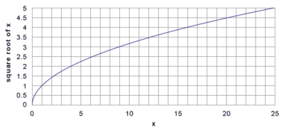
График функции 
Квадратным корнем называют также функцию  вещественной переменной , которая каждому
  ставит в соответствие арифметическое значение корня.[7] Эта функция является частным случаем степенной функции
  с
с  . Эта функция является гладкой при
  , в нуле же она непрерывна справа, но не дифференцируема.
Комплексный анализ
Обобщения
Квадратные корни вводятся как решения уравнений вида  и для других объектов: матриц [8], функций [9], операторов[10] и т. п. В качестве операции
  при этом могут использоваться достаточно произвольные мультипликативные операции, например, суперпозиция.
В алгебре применяется следующее формальное определение: Пусть  — группоид и
  . Элемент
  называется квадратным корнем из
  если
если  .
.
Квадратный корень в элементарной геометрии
Квадратные корни тесно связаны с элементарной геометрией: если дан отрезок длины 1, то с помощью циркуля и линейки можно построить те и только те отрезки, длина которых записывается выражениями, содержащими целые числа, знаки четырех действий арифметики, квадратные корни и ничего сверх того. [11]
Квадратный корень в информатике
Во многих языках программирования функционального уровня (а также языках разметки типа sqrt, от англ. square root «квадратный корень».
Алгоритмы нахождения квадратного корня
Нахождение или вычисление квадратного корня заданного числа называется извлечением (квадратного) корня.
Арифметическое извлечение квадратного корня
Для квадратов чисел верны следующие равенства:
- 1 = 12
- 1 + 3 = 22
- 1 + 3 + 5 = 32
и так далее.
То есть, узнать целую часть квадратного корня числа можно, вычитая из него все нечётные числа по порядку, пока остаток не станет меньше следующего вычитаемого числа или равен нулю, и сочтя количество выполненных действий. Например, так:
- 9 − 1 = 8
- 8 − 3 = 5
- 5 − 5 = 0
Выполнено 3 действия, квадратный корень числа 9 равен 3.
Недостатком такого способа является то, что если извлекаемый корень не является целым числом, то можно узнать только его целую часть, но не точнее. В то же время такой способ вполне доступен детям, решающим простейшие математические задачи, требующие извлечения квадратного корня.
Геометрическое извлечение квадратного корня


В частности, если  , а
, а  , то
, то  [12]
[12]
Столбиком
Этот способ позволяет найти приближённоё значение корня из любого действительного числа с любой наперёд заданной точностью.
Для ручного извлечения корня применяется запись, похожая на деление столбиком. Пусть извлекается корень из целого числа A. В отличие от деления снос производится группами по 2 цифры, причём группы следует отмечать, начиная с десятичной запятой (в обе стороны), дописывая необходимым количеством нулей.
- Найти an, квадрат которого наиболее близко подходит к группе старших разрядов числа A, оставаясь меньше последнего.
- Провести вычитание из старших разрядов A квадрата числа an.
- Удвоить an.
- Сдвинуть остаток от вычитания на 2 разряда влево, а величину 2an — на один разряд влево. Под сдвигом в данном алгоритме понимается умножение/деление на степени 10, что соответственно является сдвигом влево и вправо.
- Приписать справа от остатка вычитания два следующих старших разряда числа A.
- Сравнить полученное число с нулём.
- Если полученное число не равно 0, то найти такое 2an − 1, которое, будучи умноженным на , даст в результате число, меньшее полученного на четвёртом шаге, но наиболее близкое к нему по значению. Перейти к п.3.
- Если в п.5 получено равенство, то перейти к п.4, предварительно приписв справа от an нуль.
- После получения количества цифр, равного , прекратить вычисления (если требуется целое значение) или продолжать до необходимой точности, записывая получающиеся цифры после запятой.
 , даст в результате число, меньшее полученного на четвёртом шаге, но наиболее близкое к нему по значению. Перейти к п.3.
 , прекратить вычисления (если требуется целое значение) или продолжать до необходимой точности, записывая получающиеся цифры после запятой.
Примечания
- ↑ «Корнем n-й степени из числа x называется число, n-я степень которого совпадает с x. При n = 2 и n = 3 корни называются соответственно квадратным и кубическим.» — определение из статьи «Алгебра» энциклопедии «Кругосвет»
- ↑ «Извлечь корень n-й степени из числа а — это значит найти такое число (или числа) x, которое при возведении в n-ю степень даст данное число ()… Корень 2-й степени называется квадратным» — определение из статьи «Извлечение корня» «Большой советской энциклопедии» третьего издания.
- ↑ Теорема Лиувилля о приближении алгебраических чисел
- ↑ См. А. Я. Хинчин, Цепные дроби, М. ГИФМЛ, 1960, §§ 4, 10.
- ↑ Фихтенгольц, Григорий Михайлович. Курс дифференциального и интегрального исчисления Том. 1. Введение, § 4 // Мат. анализ на EqWorld
- ↑ Г.Корн, Т.Корн. Справочник по математике (для научных работников и инженеров). М., 1974 г., п. 1.2.1
- ↑ Фихтенгольц, гл. 2, § 1
- ↑ См., например: Гантмахер Ф. Р., Теория матриц, М.: Гос. изд-во технико-теоретической литературы, 1953, или: Воеводин В., Воеводин В., Энциклопедия линейной алгебры. Электронная система ЛИНЕАЛ, Спб.: БХВ-Петербург, 2006.
- ↑ См., например: Ершов Л. В., Райхмист Р. Б., Построение графиков функций, М.: Просвещение, 1984, или: Каплан И. А., Практические занятия по высшей математике, Харьков: Изд-во ХГУ, 1966.
- ↑ См., например: Хатсон В., Пим Дж., Приложения функционального анализа и теории операторов, М.: Мир, 1983, или: Халмош П., Гильбертово пространство в задачах, М.: Мир, 1970.
- ↑ Р. Курант Г. Роббинс Что такое математика? МЦНМО, 2000. (ГЛАВА III Геометрические построения. Алгебра числовых полей)
- ↑ Р. Курант Г. Роббинс Что такое математика? МЦНМО, 2000. Стр. 148
 )… Корень 2-й степени называется квадратным» — определение из статьи «Извлечение корня» «Большой советской энциклопедии» третьего издания.
См. также
- Корень (значения)
- Арифметический корень
- Квадратное уравнение
- Итерационная формула Герона
- Корень квадратного уравнения
- Теорема Абеля — Руффини
Ссылки
- Алгоритмы вычисления квадратного корня
- A geometric view of the square root algorithm
- Соловьев Ю., Старый алгоритм
Wikimedia Foundation.
2010.
Notation for the (principal) square root of x.
For example, √25 = 5, since 25 = 5 ⋅ 5, or 52 (5 squared).
In mathematics, a square root of a number x is a number y such that y2 = x; in other words, a number y whose square (the result of multiplying the number by itself, or y ⋅ y) is x.[1] For example, 4 and −4 are square roots of 16, because 42 = (−4)2 = 16.
Every nonnegative real number x has a unique nonnegative square root, called the principal square root, which is denoted by where the symbol is called the radical sign[2] or radix. For example, to express the fact that the principal square root of 9 is 3, we write . The term (or number) whose square root is being considered is known as the radicand. The radicand is the number or expression underneath the radical sign, in this case 9. For nonnegative x, the principal square root can also be written in exponent notation, as x1/2.
Every positive number x has two square roots: which is positive, and which is negative. The two roots can be written more concisely using the ± sign as . Although the principal square root of a positive number is only one of its two square roots, the designation «the square root» is often used to refer to the principal square root.[3][4]
Square roots of negative numbers can be discussed within the framework of complex numbers. More generally, square roots can be considered in any context in which a notion of the «square» of a mathematical object is defined. These include function spaces and square matrices, among other mathematical structures.
History
The Yale Babylonian Collection YBC 7289 clay tablet was created between 1800 BC and 1600 BC, showing and respectively as 1;24,51,10 and 0;42,25,35 base 60 numbers on a square crossed by two diagonals.[5] (1;24,51,10) base 60 corresponds to 1.41421296, which is a correct value to 5 decimal points (1.41421356…).
The Rhind Mathematical Papyrus is a copy from 1650 BC of an earlier Berlin Papyrus and other texts – possibly the Kahun Papyrus – that shows how the Egyptians extracted square roots by an inverse proportion method.[6]
In Ancient India, the knowledge of theoretical and applied aspects of square and square root was at least as old as the Sulba Sutras, dated around 800–500 BC (possibly much earlier).[citation needed] A method for finding very good approximations to the square roots of 2 and 3 are given in the Baudhayana Sulba Sutra.[7] Aryabhata, in the Aryabhatiya (section 2.4), has given a method for finding the square root of numbers having many digits.
It was known to the ancient Greeks that square roots of positive integers that are not perfect squares are always irrational numbers: numbers not expressible as a ratio of two integers (that is, they cannot be written exactly as , where m and n are integers). This is the theorem Euclid X, 9, almost certainly due to Theaetetus dating back to circa 380 BC.[8]
The particular case of the square root of 2 is assumed to date back earlier to the Pythagoreans, and is traditionally attributed to Hippasus.[citation needed] It is exactly the length of the diagonal of a square with side length 1.
In the Chinese mathematical work Writings on Reckoning, written between 202 BC and 186 BC during the early Han Dynasty, the square root is approximated by using an «excess and deficiency» method, which says to «…combine the excess and deficiency as the divisor; (taking) the deficiency numerator multiplied by the excess denominator and the excess numerator times the deficiency denominator, combine them as the dividend.»[9]
A symbol for square roots, written as an elaborate R, was invented by Regiomontanus (1436–1476). An R was also used for radix to indicate square roots in Gerolamo Cardano’s Ars Magna.[10]
According to historian of mathematics D.E. Smith, Aryabhata’s method for finding the square root was first introduced in Europe by Cataneo—in 1546.
According to Jeffrey A. Oaks, Arabs used the letter jīm/ĝīm (ج), the first letter of the word «جذر» (variously transliterated as jaḏr, jiḏr, ǧaḏr or ǧiḏr, «root»), placed in its initial form (ﺟ) over a number to indicate its square root. The letter jīm resembles the present square root shape. Its usage goes as far as the end of the twelfth century in the works of the Moroccan mathematician Ibn al-Yasamin.[11]
The symbol «√» for the square root was first used in print in 1525, in Christoph Rudolff’s Coss.[12]
Properties and uses
The graph of the function f(x) = √x, made up of half a parabola with a vertical directrix
The principal square root function (usually just referred to as the «square root function») is a function that maps the set of nonnegative real numbers onto itself. In geometrical terms, the square root function maps the area of a square to its side length.
The square root of x is rational if and only if x is a rational number that can be represented as a ratio of two perfect squares. (See square root of 2 for proofs that this is an irrational number, and quadratic irrational for a proof for all non-square natural numbers.) The square root function maps rational numbers into algebraic numbers, the latter being a superset of the rational numbers).
For all real numbers x,
- (see absolute value)
For all nonnegative real numbers x and y,
and
The square root function is continuous for all nonnegative x, and differentiable for all positive x. If f denotes the square root function, whose derivative is given by:
The Taylor series of about x = 0 converges for |x| ≤ 1, and is given by
The square root of a nonnegative number is used in the definition of Euclidean norm (and distance), as well as in generalizations such as Hilbert spaces. It defines an important concept of standard deviation used in probability theory and statistics. It has a major use in the formula for roots of a quadratic equation; quadratic fields and rings of quadratic integers, which are based on square roots, are important in algebra and have uses in geometry. Square roots frequently appear in mathematical formulas elsewhere, as well as in many physical laws.
Square roots of positive integers
A positive number has two square roots, one positive, and one negative, which are opposite to each other. When talking of the square root of a positive integer, it is usually the positive square root that is meant.
The square roots of an integer are algebraic integers—more specifically quadratic integers.
The square root of a positive integer is the product of the roots of its prime factors, because the square root of a product is the product of the square roots of the factors. Since only roots of those primes having an odd power in the factorization are necessary. More precisely, the square root of a prime factorization is
As decimal expansions
The square roots of the perfect squares (e.g., 0, 1, 4, 9, 16) are integers. In all other cases, the square roots of positive integers are irrational numbers, and hence have non-repeating decimals in their decimal representations. Decimal approximations of the square roots of the first few natural numbers are given in the following table.
-
n truncated to 50 decimal places
0 0 1 1 2 1.41421356237309504880168872420969807856967187537694 3 1.73205080756887729352744634150587236694280525381038 4 2 5 2.23606797749978969640917366873127623544061835961152 6 2.44948974278317809819728407470589139196594748065667 7 2.64575131106459059050161575363926042571025918308245 8 2.82842712474619009760337744841939615713934375075389 9 3 10 3.16227766016837933199889354443271853371955513932521
As expansions in other numeral systems
As with before, the square roots of the perfect squares (e.g., 0, 1, 4, 9, 16) are integers. In all other cases, the square roots of positive integers are irrational numbers, and therefore have non-repeating digits in any standard positional notation system.
The square roots of small integers are used in both the SHA-1 and SHA-2 hash function designs to provide nothing up my sleeve numbers.
As periodic continued fractions
One of the most intriguing results from the study of irrational numbers as continued fractions was obtained by Joseph Louis Lagrange c. 1780. Lagrange found that the representation of the square root of any non-square positive integer as a continued fraction is periodic. That is, a certain pattern of partial denominators repeats indefinitely in the continued fraction. In a sense these square roots are the very simplest irrational numbers, because they can be represented with a simple repeating pattern of integers.
-
= [1; 2, 2, …] = [1; 1, 2, 1, 2, …] = [2] = [2; 4, 4, …] = [2; 2, 4, 2, 4, …] = [2; 1, 1, 1, 4, 1, 1, 1, 4, …] = [2; 1, 4, 1, 4, …] = [3] = [3; 6, 6, …] = [3; 3, 6, 3, 6, …] = [3; 2, 6, 2, 6, …] = [3; 1, 1, 1, 1, 6, 1, 1, 1, 1, 6, …] = [3; 1, 2, 1, 6, 1, 2, 1, 6, …] = [3; 1, 6, 1, 6, …] = [4] = [4; 8, 8, …] = [4; 4, 8, 4, 8, …] = [4; 2, 1, 3, 1, 2, 8, 2, 1, 3, 1, 2, 8, …] = [4; 2, 8, 2, 8, …]
The square bracket notation used above is a short form for a continued fraction. Written in the more suggestive algebraic form, the simple continued fraction for the square root of 11, [3; 3, 6, 3, 6, …], looks like this:
where the two-digit pattern {3, 6} repeats over and over again in the partial denominators. Since 11 = 32 + 2, the above is also identical to the following generalized continued fractions:
Computation
Square roots of positive numbers are not in general rational numbers, and so cannot be written as a terminating or recurring decimal expression. Therefore in general any attempt to compute a square root expressed in decimal form can only yield an approximation, though a sequence of increasingly accurate approximations can be obtained.
Most pocket calculators have a square root key. Computer spreadsheets and other software are also frequently used to calculate square roots. Pocket calculators typically implement efficient routines, such as the Newton’s method (frequently with an initial guess of 1), to compute the square root of a positive real number.[13][14] When computing square roots with logarithm tables or slide rules, one can exploit the identities
where ln and log10 are the natural and base-10 logarithms.
By trial-and-error,[15] one can square an estimate for and raise or lower the estimate until it agrees to sufficient accuracy. For this technique it is prudent to use the identity
as it allows one to adjust the estimate x by some amount c and measure the square of the adjustment in terms of the original estimate and its square. Furthermore, (x + c)2 ≈ x2 + 2xc when c is close to 0, because the tangent line to the graph of x2 + 2xc + c2 at c = 0, as a function of c alone, is y = 2xc + x2. Thus, small adjustments to x can be planned out by setting 2xc to a, or c = a/(2x).
The most common iterative method of square root calculation by hand is known as the «Babylonian method» or «Heron’s method» after the first-century Greek philosopher Heron of Alexandria, who first described it.[16]
The method uses the same iterative scheme as the Newton–Raphson method yields when applied to the function y = f(x) = x2 − a, using the fact that its slope at any point is dy/dx = f′(x) = 2x, but predates it by many centuries.[17]
The algorithm is to repeat a simple calculation that results in a number closer to the actual square root each time it is repeated with its result as the new input. The motivation is that if x is an overestimate to the square root of a nonnegative real number a then a/x will be an underestimate and so the average of these two numbers is a better approximation than either of them. However, the inequality of arithmetic and geometric means shows this average is always an overestimate of the square root (as noted below), and so it can serve as a new overestimate with which to repeat the process, which converges as a consequence of the successive overestimates and underestimates being closer to each other after each iteration. To find x:
- Start with an arbitrary positive start value x. The closer to the square root of a, the fewer the iterations that will be needed to achieve the desired precision.
- Replace x by the average (x + a/x) / 2 between x and a/x.
- Repeat from step 2, using this average as the new value of x.
That is, if an arbitrary guess for is x0, and xn + 1 = (xn + a/xn) / 2, then each xn is an approximation of which is better for large n than for small n. If a is positive, the convergence is quadratic, which means that in approaching the limit, the number of correct digits roughly doubles in each next iteration. If a = 0, the convergence is only linear.
Using the identity
the computation of the square root of a positive number can be reduced to that of a number in the range [1,4). This simplifies finding a start value for the iterative method that is close to the square root, for which a polynomial or piecewise-linear approximation can be used.
The time complexity for computing a square root with n digits of precision is equivalent to that of multiplying two n-digit numbers.
Another useful method for calculating the square root is the shifting nth root algorithm, applied for n = 2.
The name of the square root function varies from programming language to programming language, with sqrt[18] (often pronounced «squirt» [19]) being common, used in C, C++, and derived languages like JavaScript, PHP, and Python.
Square roots of negative and complex numbers
First leaf of the complex square root
Second leaf of the complex square root
Using the Riemann surface of the square root, it is shown how the two leaves fit together
The square of any positive or negative number is positive, and the square of 0 is 0. Therefore, no negative number can have a real square root. However, it is possible to work with a more inclusive set of numbers, called the complex numbers, that does contain solutions to the square root of a negative number. This is done by introducing a new number, denoted by i (sometimes written as j, especially in the context of electricity where «i» traditionally represents electric current) and called the imaginary unit, which is defined such that i2 = −1. Using this notation, we can think of i as the square root of −1, but we also have (−i)2 = i2 = −1 and so −i is also a square root of −1. By convention, the principal square root of −1 is i, or more generally, if x is any nonnegative number, then the principal square root of −x is
The right side (as well as its negative) is indeed a square root of −x, since
For every non-zero complex number z there exist precisely two numbers w such that w2 = z: the principal square root of z (defined below), and its negative.
Principal square root of a complex number
Geometric representation of the 2nd to 6th roots of a complex number z, in polar form reiφ where r = |z | and φ = arg z. If z is real, φ = 0 or π. Principal roots are shown in black.
To find a definition for the square root that allows us to consistently choose a single value, called the principal value, we start by observing that any complex number can be viewed as a point in the plane, expressed using Cartesian coordinates. The same point may be reinterpreted using polar coordinates as the pair where is the distance of the point from the origin, and is the angle that the line from the origin to the point makes with the positive real () axis. In complex analysis, the location of this point is conventionally written If
then the principal square root of is defined to be the following:
The principal square root function is thus defined using the nonpositive real axis as a branch cut.
If is a non-negative real number (which happens if and only if ) then the principal square root of is in other words, the principal square root of a non-negative real number is just the usual non-negative square root.
It is important that because if, for example, (so ) then the principal square root is
but using would instead produce the other square root
The principal square root function is holomorphic everywhere except on the set of non-positive real numbers (on strictly negative reals it is not even continuous). The above Taylor series for remains valid for complex numbers with
The above can also be expressed in terms of trigonometric functions:
Algebraic formula
When the number is expressed using its real and imaginary parts, the following formula can be used for the principal square root:[20][21]
where sgn(y) is the sign of y (except that, here, sgn(0) = 1). In particular, the imaginary parts of the original number and the principal value of its square root have the same sign. The real part of the principal value of the square root is always nonnegative.
For example, the principal square roots of ±i are given by:
Notes
In the following, the complex z and w may be expressed as:
where and .
Because of the discontinuous nature of the square root function in the complex plane, the following laws are not true in general.
A similar problem appears with other complex functions with branch cuts, e.g., the complex logarithm and the relations logz + logw = log(zw) or log(z*) = log(z)* which are not true in general.
Wrongly assuming one of these laws underlies several faulty «proofs», for instance the following one showing that −1 = 1:
The third equality cannot be justified (see invalid proof).[22]: Chapter VI Some fallacies in algebra and trigonometry, Section I The fallacies, Subsection 2 The fallacy that +1 = -1 It can be made to hold by changing the meaning of √ so that this no longer represents the principal square root (see above) but selects a branch for the square root that contains The left-hand side becomes either
if the branch includes +i or
if the branch includes −i, while the right-hand side becomes
where the last equality, is a consequence of the choice of branch in the redefinition of √.
Nth roots and polynomial roots
The definition of a square root of as a number such that has been generalized in the following way.
A cube root of is a number such that ; it is denoted
If n is an integer greater than two, a nth root of is a number such that ; it is denoted
Given any polynomial p, a root of p is a number y such that p(y) = 0. For example, the nth roots of x are the roots of the polynomial (in y)
Abel–Ruffini theorem states that, in general, the roots of a polynomial of degree five or higher cannot be expressed in terms of nth roots.
Square roots of matrices and operators
If A is a positive-definite matrix or operator, then there exists precisely one positive definite matrix or operator B with B2 = A; we then define A1/2 = B. In general matrices may have multiple square roots or even an infinitude of them. For example, the 2 × 2 identity matrix has an infinity of square roots,[23] though only one of them is positive definite.
In integral domains, including fields
Each element of an integral domain has no more than 2 square roots. The difference of two squares identity u2 − v2 = (u − v)(u + v) is proved using the commutativity of multiplication. If u and v are square roots of the same element, then u2 − v2 = 0. Because there are no zero divisors this implies u = v or u + v = 0, where the latter means that two roots are additive inverses of each other. In other words if an element a square root u of an element a exists, then the only square roots of a are u and −u. The only square root of 0 in an integral domain is 0 itself.
In a field of characteristic 2, an element either has one square root or does not have any at all, because each element is its own additive inverse, so that −u = u. If the field is finite of characteristic 2 then every element has a unique square root. In a field of any other characteristic, any non-zero element either has two square roots, as explained above, or does not have any.
Given an odd prime number p, let q = pe for some positive integer e. A non-zero element of the field Fq with q elements is a quadratic residue if it has a square root in Fq. Otherwise, it is a quadratic non-residue. There are (q − 1)/2 quadratic residues and (q − 1)/2 quadratic non-residues; zero is not counted in either class. The quadratic residues form a group under multiplication. The properties of quadratic residues are widely used in number theory.
In rings in general
Unlike in an integral domain, a square root in an arbitrary (unital) ring need not be unique up to sign. For example, in the ring of integers modulo 8 (which is commutative, but has zero divisors), the element 1 has four distinct square roots: ±1 and ±3.
Another example is provided by the ring of quaternions which has no zero divisors, but is not commutative. Here, the element −1 has infinitely many square roots, including ±i, ±j, and ±k. In fact, the set of square roots of −1 is exactly
A square root of 0 is either 0 or a zero divisor. Thus in rings where zero divisors do not exist, it is uniquely 0. However, rings with zero divisors may have multiple square roots of 0. For example, in any multiple of n is a square root of 0.
Geometric construction of the square root
The square root of a positive number is usually defined as the side length of a square with the area equal to the given number. But the square shape is not necessary for it: if one of two similar planar Euclidean objects has the area a times greater than another, then the ratio of their linear sizes is .
A square root can be constructed with a compass and straightedge. In his Elements, Euclid (fl. 300 BC) gave the construction of the geometric mean of two quantities in two different places: Proposition II.14 and Proposition VI.13. Since the geometric mean of a and b is , one can construct simply by taking b = 1.
The construction is also given by Descartes in his La Géométrie, see figure 2 on page 2. However, Descartes made no claim to originality and his audience would have been quite familiar with Euclid.
Euclid’s second proof in Book VI depends on the theory of similar triangles. Let AHB be a line segment of length a + b with AH = a and HB = b. Construct the circle with AB as diameter and let C be one of the two intersections of the perpendicular chord at H with the circle and denote the length CH as h. Then, using Thales’ theorem and, as in the proof of Pythagoras’ theorem by similar triangles, triangle AHC is similar to triangle CHB (as indeed both are to triangle ACB, though we don’t need that, but it is the essence of the proof of Pythagoras’ theorem) so that AH:CH is as HC:HB, i.e. a/h = h/b, from which we conclude by cross-multiplication that h2 = ab, and finally that . When marking the midpoint O of the line segment AB and drawing the radius OC of length (a + b)/2, then clearly OC > CH, i.e. (with equality if and only if a = b), which is the arithmetic–geometric mean inequality for two variables and, as noted above, is the basis of the Ancient Greek understanding of «Heron’s method».
Another method of geometric construction uses right triangles and induction: can be constructed, and once has been constructed, the right triangle with legs 1 and has a hypotenuse of . Constructing successive square roots in this manner yields the Spiral of Theodorus depicted above.
See also
- Apotome (mathematics)
- Cube root
- Functional square root
- Integer square root
- Nested radical
- Nth root
- Root of unity
- Solving quadratic equations with continued fractions
- Square root principle
- Quantum gate § Square root of NOT gate (√NOT)
Notes
- ^ Gel’fand, p. 120 Archived 2016-09-02 at the Wayback Machine
- ^ «Squares and Square Roots». www.mathsisfun.com. Retrieved 2020-08-28.
- ^ Zill, Dennis G.; Shanahan, Patrick (2008). A First Course in Complex Analysis With Applications (2nd ed.). Jones & Bartlett Learning. p. 78. ISBN 978-0-7637-5772-4. Archived from the original on 2016-09-01. Extract of page 78 Archived 2016-09-01 at the Wayback Machine
- ^ Weisstein, Eric W. «Square Root». mathworld.wolfram.com. Retrieved 2020-08-28.
- ^ «Analysis of YBC 7289». ubc.ca. Retrieved 19 January 2015.
- ^ Anglin, W.S. (1994). Mathematics: A Concise History and Philosophy. New York: Springer-Verlag.
- ^ Joseph, ch.8.
- ^ Heath, Sir Thomas L. (1908). The Thirteen Books of The Elements, Vol. 3. Cambridge University Press. p. 3.
- ^ Dauben (2007), p. 210.
- ^ «The Development of Algebra — 2». maths.org. Archived from the original on 24 November 2014. Retrieved 19 January 2015.
- ^ * Oaks, Jeffrey A. (2012). Algebraic Symbolism in Medieval Arabic Algebra (PDF) (Thesis). Philosophica. p. 36. Archived (PDF) from the original on 2016-12-03.
- ^ Manguel, Alberto (2006). «Done on paper: the dual nature of numbers and the page». The Life of Numbers. ISBN 84-86882-14-1.
- ^ Parkhurst, David F. (2006). Introduction to Applied Mathematics for Environmental Science. Springer. pp. 241. ISBN 9780387342283.
- ^ Solow, Anita E. (1993). Learning by Discovery: A Lab Manual for Calculus. Cambridge University Press. pp. 48. ISBN 9780883850831.
- ^ Aitken, Mike; Broadhurst, Bill; Hladky, Stephen (2009). Mathematics for Biological Scientists. Garland Science. p. 41. ISBN 978-1-136-84393-8. Archived from the original on 2017-03-01. Extract of page 41 Archived 2017-03-01 at the Wayback Machine
- ^ Heath, Sir Thomas L. (1921). A History of Greek Mathematics, Vol. 2. Oxford: Clarendon Press. pp. 323–324.
- ^ Muller, Jean-Mic (2006). Elementary functions: algorithms and implementation. Springer. pp. 92–93. ISBN 0-8176-4372-9., Chapter 5, p 92 Archived 2016-09-01 at the Wayback Machine
- ^ «Function sqrt». CPlusPlus.com. The C++ Resources Network. 2016. Archived from the original on November 22, 2012. Retrieved June 24, 2016.
- ^ Overland, Brian (2013). C++ for the Impatient. Addison-Wesley. p. 338. ISBN 9780133257120. OCLC 850705706. Archived from the original on September 1, 2016. Retrieved June 24, 2016.
- ^ Abramowitz, Milton; Stegun, Irene A. (1964). Handbook of mathematical functions with formulas, graphs, and mathematical tables. Courier Dover Publications. p. 17. ISBN 0-486-61272-4. Archived from the original on 2016-04-23., Section 3.7.27, p. 17 Archived 2009-09-10 at the Wayback Machine
- ^ Cooke, Roger (2008). Classical algebra: its nature, origins, and uses. John Wiley and Sons. p. 59. ISBN 978-0-470-25952-8. Archived from the original on 2016-04-23.
- ^ Maxwell, E. A. (1959). Fallacies in Mathematics. Cambridge University Press.
- ^ Mitchell, Douglas W., «Using Pythagorean triples to generate square roots of I2«, Mathematical Gazette 87, November 2003, 499–500.
References
- Dauben, Joseph W. (2007). «Chinese Mathematics I». In Katz, Victor J. (ed.). The Mathematics of Egypt, Mesopotamia, China, India, and Islam. Princeton: Princeton University Press. ISBN 978-0-691-11485-9.
- Gel’fand, Izrael M.; Shen, Alexander (1993). Algebra (3rd ed.). Birkhäuser. p. 120. ISBN 0-8176-3677-3.
- Joseph, George (2000). The Crest of the Peacock. Princeton: Princeton University Press. ISBN 0-691-00659-8.
- Smith, David (1958). History of Mathematics. Vol. 2. New York: Dover Publications. ISBN 978-0-486-20430-7.
- Selin, Helaine (2008), Encyclopaedia of the History of Science, Technology, and Medicine in Non-Western Cultures, Springer, Bibcode:2008ehst.book…..S, ISBN 978-1-4020-4559-2.
External links
- Algorithms, implementations, and more – Paul Hsieh’s square roots webpage
- How to manually find a square root
- AMS Featured Column, Galileo’s Arithmetic by Tony Philips – includes a section on how Galileo found square roots
На данной странице описаны правила ввода функций, которых следует придерживаться в онлайн калькуляторах для решения производных и решения интегралов.
Не забывайте проверять правильность написания формул. Неточность и ошибки в написании, приводят к неверному ответу и ситуациям, при которых калькулятор отказывается проводить вычисления.
|
Оператор |
Описание |
|
Простейшие математические операции |
|
|
+ — * / () |
Сложение, вычитание, умножение, деление и группирующие символы. Знак умножения * — необязателен: выражение 2sin(3 x ) эквивалентно 2*sin(3* x ). |
|
0.5 |
Десятичные дроби записываются через точку:
|
|
Элементарные функции |
|
|
x ^ n |
Возведение в степень:
xn , например x ^2 значит x 2 |
|
sqrt( x ) |
Квадратный корень: √
x . Эквивалентно root(x ,2) или x ^(1/2) |
|
cbrt( x ) |
Кубический корень: 3√
x . Эквивалентно root(x ,3) или x ^(1/3) |
|
root( x , n ) |
Корень
n -той степени из x . Эквивалентно x ^(1/ n ) |
|
log( a , x ) |
Логарифм от
x по основанию a |
|
ln( x ) |
Натуральный логарифм (логарифм c основанием
e ) |
|
lg( x ) |
Десятичный логарифм (логарифм по основанию 10) |
|
exp( x ) |
Экспоненциальная функция, эквивалентно
e ^ x |
|
Тригонометрические функции |
|
|
sin( x ) |
Синус от
x |
|
cos( x ) |
Косинус от
x |
|
tg( x ) |
Тангенс от
x . Можно вводить tg( x ) или tan( x ) |
|
ctg( x ) |
Котангенс от
x . Можно вводить ctg( x ) или cot( x ) |
|
sec( x ) |
Секанс от
x , определяется как 1/cos( x ) |
|
csc( x ) |
Косеканс от
x , определяется как 1/sin( x ) |
|
arcsin( x ) |
Арксинус от
x . Можно вводить arcsin( x ) или asin( x ) |
|
arccos( x ) |
Арккосинус от
x . Можно вводить arccos( x ) или acos( x ) |
|
atan( x ) |
Арктангенс от
x . Можно вводить arctg( x ) или atan( x ) |
|
arcctg( x ) |
Арккотангенс от
x . Можно вводить arcctg( x ) или acot( x ) |
|
asec( x ) |
Арксеканс от
x |
|
acsc( x ) |
Арккосеканс от
x |
|
Некоторые константы |
|
|
e |
Число Эйлера
e = 2.718281828459045… |
|
pi |
Число
π = 3.141592653589793… |
5 способов поставить знак корня на компьютере в ворде и других программах, на телефоне и планшете
Просмотров 55.1к. Опубликовано 29.06.2020 Обновлено 04.10.2021
Есть символы, которые используются редко и, кажется, что на компьютере их поставить невозможно. Проще распечатать документ, вписать их вручную, или использовать какое-то буквенное обозначение. Среди таких элементов – квадратный корень √. Найти значок корня на клавиатуре невозможно. Но это не означает, что ставить его нельзя. Читайте нашу статью, в ней мы готовы показать вам, как любую математическую, физическую запись сделать изящной и красивой на пк, ноутбуке, телефоне.
Содержание
- Где в компьютере используется квадратный корень √
- Способы набора корня на клавиатуре компьютера и ноутбука
- Используем таблицу символов
- Код символа
- Значок корня в уравнении
- Шестнадцатеричный код
- Способы набора символа в ворде
- На телефоне
- Проблемы со вставкой символа корня
- Выводы
Где в компьютере используется квадратный корень √
 Корень – математический символ. Иногда он также называется радикалом. Элемент не нашел большого применения в ежедневной жизни обычного человека. Применяется при подготовке специальных работ, документов, когда огромные формулы, многошаговые уравнения, вычисления можно выразить изящно и аккуратно при помощи математических элементов.
Среди таких работ:
- дипломы по математике;
- курсовые по алгебре, информатике;
- инженерные расчеты;
- запись результатов исследований по физике:
- калькуляции строительных, ремонтных работ;
- научные исследования.
Способы набора корня на клавиатуре компьютера и ноутбука
Часто, чтобы поставить в текст радикал или запись с ним, используются сочетания букв. Sqrt, например, означает кв. корень, а cbrt – кубический. Но писать буквенные комбинации, слова неудобно. Кроме того, они не всем понятны.
Удобнее использовать известный элемент √, похожий на галочку с одной длинной стороной. Способов вставить в текст его не так много. О каждом мы сейчас подробно расскажем.
Используем таблицу символов