Определение натурального числа
Натуральные числа — это числа, которые мы используем для подсчета чего-то конкретного, осязаемого.
Вот какие числа называют натуральными: 1, 2, 3, 4, 5, 6, 7, 8, 9, 10, 11, 12, 13 и т. д.
Натуральный ряд — последовательность всех натуральных чисел, расположенных в порядке возрастания. Первые сто можно посмотреть в таблице.
| Особенности натуральных чисел |
|---|
|
Какие операции возможны над натуральными числами
- сложение:
слагаемое + слагаемое = сумма; - умножение:
множитель × множитель = произведение; - вычитание:
уменьшаемое − вычитаемое = разность.При этом уменьшаемое должно быть больше вычитаемого, иначе в результате получится отрицательное число или ноль;
- деление:
делимое : делитель = частное; - деление с остатком:
делимое / делитель = частное (остаток); - возведение в степень:
ab, где a — основание степени, b — показатель степени.
Записывайтесь на курсы обучения математике для учеников с 1 по 11 классы!
Получай лайфхаки, статьи, видео и чек-листы по обучению на почту
Реши домашку по математике на 5.
Подробные решения помогут разобраться в самой сложной теме.
Десятичная запись натурального числа
В школе мы проходим тему натуральных чисел в 5 классе, но на самом деле многое нам может быть интуитивно понятно и раньше. Проговорим важные правила.
Мы регулярно используем цифры: 0, 1, 2, 3, 4, 5, 6, 7, 8, 9. При записи любого натурального числа можно использовать только эти цифры без каких-либо других символов. Записываем цифры одну за другой в строчку слева направо, используем одну высоту.
Примеры правильной записи натуральных чисел: 208, 567, 24, 1 467, 899 112. Эти примеры показывают нам, что последовательность цифр может быть разной и некоторые даже могут повторяться.
077, 0, 004, 0931 — это примеры неправильной записи натуральных чисел, потому что ноль расположен слева. Число не может начинаться с нуля. Это и есть десятичная запись натурального числа.
Количественный смысл натуральных чисел
Натуральные числа несут в себе количественный смысл, то есть выступают в качестве инструмента для нумерации.
Представим, что перед нами банан 🍌. Мы можем записать, что видим 1 банан. При этом натуральное число 1 читается как «один» или «единица».
Но термин «единица» имеет еще одно значение: то, что можно рассмотреть, как единое целое. Элемент множества можно обозначить единицей. Например, любое дерево из множества деревьев — единица, любой листок из множества листков — единица.
Представим, что перед нами 2 банана 🍌🍌. Натуральное число 2 читается как «два». Далее, по аналогии:
| 🍌🍌🍌 | 3 предмета («три») |
| 🍌🍌🍌🍌 | 4 предмета («четыре») |
| 🍌🍌🍌🍌🍌 | 5 предметов («пять») |
| 🍌🍌🍌🍌🍌🍌 | 6 предметов («шесть») |
| 🍌🍌🍌🍌🍌🍌🍌 | 7 предметов («семь») |
| 🍌🍌🍌🍌🍌🍌🍌🍌 | 8 предметов («восемь») |
| 🍌🍌🍌🍌🍌🍌🍌🍌🍌 | 9 предметов («девять») |
Основная функция натурального числа — указать количество предметов.
Если запись числа совпадает с цифрой 0, то его называют «ноль». Напомним, что ноль — не натуральное число, но он может обозначать отсутствие. Ноль предметов значит — ни одного.
Однозначные, двузначные и трехзначные натуральные числа
Однозначное натуральное число — это такое число, в составе которого один знак, одна цифра. Девять однозначных натуральных чисел: 1, 2, 3, 4, 5, 6, 7, 8, 9.
Двузначные натуральные числа — те, в составе которых два знака, две цифры. Цифры могут повторяться или быть различными. Например: 88, 53, 70.
Если множество предметов состоит из девяти и еще одного, значит, речь идет об 1 десятке («один десяток») предметов. Если один десяток и еще один, значит, перед нами 2 десятка («два десятка») и так далее.
По сути, двузначное число — это набор однозначных чисел, где одно записывается справа, а другое слева. Число слева показывает количество десятков в составе натурального числа, а число справа — количество единиц. Всего двузначных натуральных чисел — 90.
Трехзначные натуральные числа — числа, в составе которых три знака, три цифры. Например: 666, 389, 702.
Одна сотня — это множество, состоящее из десяти десятков. Сотня и еще одна сотня — 2 сотни. Прибавим еще одну сотню — 3 сотни.
Вот как происходит запись трехзначного числа: натуральные числа записываются одно за другим слева направо.
Крайнее правое однозначное число указывает на количество единиц, следующее — на количество десятков, крайнее левое — на количество сотен. Цифра 0 показывает отсутствие единиц или десятков. Поэтому 506 — это 5 сотен, 0 десятков и 6 единиц.
Точно так же определяются четырехзначные, пятизначные, шестизначные и другие натуральные числа.
Многозначные натуральные числа
Многозначные натуральные числа состоят из двух и более знаков.
1 000 — это множество с десятью сотнями, 1 000 000 состоит из тысячи тысяч, а один миллиард — это тысяча миллионов. Тысяча миллионов, только представьте! То есть мы можем рассмотреть любое многозначное натуральное число как набор однозначных натуральных чисел.
Например, 2 873 206 содержит в себе: 6 единиц, 0 десятков, 2 сотни, 3 тысячи, 7 десятков тысяч, 8 сотен тысяч и 2 миллиона.
Сколько всего натуральных чисел?
Однозначных 9, двузначных 90, трехзначных 900 и т.д.
Свойства натуральных чисел
Об особенностях натуральных чисел мы уже знаем. А теперь подробно расскажем про их свойства:
| множество натуральных чисел | бесконечно и начинается с единицы (1) |
| за каждым натуральным числом следует другое | оно больше предыдущего на 1 |
| результат деления натурального числа на единицу (1) | само натуральное число: 5 : 1 = 5 |
| результат деления натурального числа самого на себя | единица (1): 6 : 6 = 1 |
| переместительный закон сложения | от перестановки мест слагаемых сумма не меняется: 4 + 3 = 3 + 4 |
| сочетательный закон сложения | результат сложения нескольких слагаемых не зависит от порядка действий: (2 + 3) + 4 = 2 + (3 + 4) |
| переместительный закон умножения | от перестановки мест множителей произведение не изменится: 4 × 5 = 5 × 4 |
| сочетательный закон умножения | результат произведения множителей не зависит от порядка действий; можно хоть так, хоть эдак: (6 × 7) × 8 = 6 × (7 ×  |
| распределительный закон умножения относительно сложения | чтобы умножить сумму на число, нужно каждое слагаемое умножить на это число и полученные результаты сложить: 4 × (5 + 6) = 4 × 5 + 4 × 6 |
| распределительный закон умножения относительно вычитания | чтобы умножить разность на число, можно умножить на это число отдельно уменьшаемое и вычитаемое, а затем из первого произведения вычесть второе: 3 × (4 − 5) = 3 × 4 − 3 × 5 |
| распределительный закон деления относительно сложения | чтобы разделить сумму на число, можно разделить на это число каждое слагаемое и сложить полученные результаты: (9 + : 3 = 9 : 3 + 8 : 3 |
| распределительный закон деления относительно вычитания | чтобы разделить разность на число, можно разделить на это число сначала уменьшаемое, а затем вычитаемое, и из первого произведения вычесть второе: (5 − 3) : 2 = 5 : 2 − 3 : 2 |
Разряды натурального числа и значение разряда
Напомним, что от позиции, на которой стоит цифра в записи числа, зависит ее значение. Так, например, 1 123 содержит в себе: 3 единицы, 2 десятка, 1 сотню, 1 тысячу. При этом можно сформулировать иначе и сказать, что в заданном числе 1 123 цифра 3 располагается в разряде единиц, 2 в разряде десятков, 1 в разряде сотен и 1 служит значением разряда тысяч.
Разряд — это позиция, место расположения цифры в записи натурального числа.
У каждого разряда есть свое название. Слева всегда располагаются старшие разряды, а справа — младшие. Чтобы быстрее запомнить, можно использовать таблицу.
Количество разрядов всегда соответствует количеству знаков в числе. В этой таблице есть названия всех разрядов для числа, которое состоит из 15 знаков. У следующих разрядов также есть названия, но они используются крайне редко.
Низший (младший) разряд многозначного натурального числа — разряд единиц.
Высший (старший) разряд многозначного натурального числа — разряд, соответствующий крайней левой цифре в заданном числе.
Вы наверняка заметили, что в учебниках часто ставят небольшие пробелы при записи многозначных чисел. Так делают, чтобы натуральные числа было удобно читать. А еще — чтобы визуально разделить разные классы чисел.
Класс — это группа разрядов, которая содержит в себе три разряда: единицы, десятки и сотни.
Десятичная система счисления
Люди в разные времена использовали разные методы записи чисел. И каждая система счисления имеет свои правила и особенности.
Десятичная система счисления — самая распространенная система счисления, в которой для записи чисел используют десять знаков: 0, 1, 2, 3, 4, 5, 6, 7, 8, 9.
В десятичной системе значение одной и той же цифры зависит от ее позиции в записи числа. Например, число 555 состоит из трех одинаковых цифр. В этом числе первая слева цифра означает пять сотен, вторая — пять десятков, а третья — пять единиц. Так как значение цифры зависит от ее позиции, десятичную систему счисления называют позиционной.
Вопрос для самопроверки
Сколько натуральных чисел можно отметить на координатном луче между точками с координатами:
-
0 и 15;
-
20 и 50;
-
100 и 130?
Из большого количества разнообразных множеств особо интересными и важными являются числовые множества, т.е. те множества, элементами которых служат числа. Очевидно, что для работы с числовыми множествами необходимо иметь навык записи их, а также изображения их на координатной прямой.
Запись числовых множеств
Общепринятым обозначением любых множеств являются заглавные буквы латиницы. Числовые множества – не исключение. К примеру, мы можем говорить о числовых множествах B, F или S и т.п. Однако есть также общепринятая маркировка числовых множеств в зависимости от входящих в него элементов:
N – множество всех натуральных чисел; Z – множество целых чисел; Q – множество рациональных чисел; J – множество иррациональных чисел; R – множество действительных чисел; C – множество комплексных чисел.
Становится понятным, что обозначение, например, множества, состоящего из двух чисел: -3, 8 буквой J может ввести в заблуждение, поскольку этой буквой маркируется множество иррациональных чисел. Поэтому для обозначения множества -3, 8 более подходящим будет использование какой-то нейтральной буквы: A или B, например.
Напомним также следующие обозначения:
- ∅ – пустое множество или множество, не имеющее составных элементов;
- ∈ или ∉ — знак принадлежности или непринадлежности элемента множеству. Например, запись 5 ∈ N обозначает, что число 5 является частью множества всех натуральных чисел. Запись -7,1 ∈ Z отражает тот факт, что число -7,1 не является элементом множества Z, т.к. Z– множество целых чисел;
- знаки принадлежности множества множеству:
⊂ или ⊃ — знаки «включено» или «включает» соответственно. Например, запись A⊂Z означает, что все элементы множества А входят в множество Z, т.е. числовое множество A включено в множество Z. Или наоборот, запись Z⊃A пояснит, что множество всех целых чисел Z включает множество A.
⊆ или ⊇ — знаки так называемого нестрогого включения. Означают «включено или совпадает» и «включает или совпадает» соответственно.
Рассмотрим теперь схему описания числовых множеств на примере основных стандартных случаев, наиболее часто используемых на практике.
Первыми рассмотрим числовые множества, содержащие конечное и небольшое количество элементов. Описание подобного множества удобно составлять, просто перечисляя все его элементы. Элементы в виде чисел записываются, разделяясь запятой, и заключаются в фигурные скобки (что соответствует общим правилам описания множеств). К примеру, множество из чисел 8, -17, 0,15 запишем как {8, -17, 0,15}.
Случается, что количество элементов множества достаточно велико, но все они подчиняются определенной закономерности: тогда в описании множества используют многоточие. К примеру, множество всех четных чисел от 2 до 88 запишем как: {2, 4, 6, 8, …, 88}.
Теперь поговорим об описании числовых множеств, в которых количество элементов бесконечно. Иногда их описывают при помощи того же многоточия. Например, множество всех натуральных чисел запишем так: N = {1, 2, 3, …}.
Также возможно записать числовое множество с бесконечным количеством элементов при помощи указания свойств его элементов. Применяют при этом обозначение {х| свойства}. К примеру, {n| 8·n + 3, n∈N} определяет множество натуральных чисел, которые при делении на 8 дадут остаток 3. Это же множество возможно записать как: {11, 19, 27, …}.
В частных случаях числовые множества с бесконечным количеством элементов – это общеизвестные множества N, Z, R и т.д., либо числовые промежутки. Но в основном числовые множества представляют собой объединение составляющих их числовых промежутков и числовых множеств с конечным количеством элементов (о них мы говорили в самом начале статьи).
Рассмотрим на примере. Допустим, составляющими некого числового множества являются числа -15, -8, -7,34, 0, а также все числа отрезка [-6, -1,2] и числа открытого числового луча (6, +∞). В соответствии с определением объединения множеств заданное числовое множество запишем как: {-15, -8, -7,34}∪[-6, -1,2]∪{0}∪(6, +∞). Подобная запись фактически означает множество, включающее в себя все элементы множеств {-15, -8, -7,34, 0}, [-6, -1,2] и (6, +∞).
Таким же образом, объединяя различные числовые промежутки и множества отдельных чисел, возможно дать описание любому числовому множеству, состоящему из действительных чисел. На основе сказанного становится понятно, для чего вводятся различные виды числовых промежутков, такие как интервал, полуинтервал, отрезок, открытый числовой луч и числовой луч. Все эти виды промежутков совместно с обозначениями множеств отдельных чисел дают возможность через их объединение описать любое числовое множество.
Необходимо также обратить внимание на то, что отдельные числа и числовые промежутки при записи множества могут быть упорядочены по возрастанию. В общем, это не является обязательным требованием, однако подобное упорядочивание позволяет представить числовое множество проще, а также верно отобразить его на координатной прямой. Также стоит уточнить, что в таких записях не применяют числовые промежутки с общими элементами, поскольку эти записи возможно заменить объединением числовых промежутков, исключив общие элементы. К примеру, объединением числовых множеств с общими элементами [-15, 0] и (-6,4) будет полуинтервал [-15, 4). То же имеет отношение и к объединению числовых промежутков с одинаковыми граничными числами. Например, объединение (4, 7]∪(7, 9] является множеством (4, 9]. Этот пункт подробно будет рассмотрен в теме нахождения пересечения и объединения числовых множеств.
Изображение числовых множеств на координатной прямой
В практических примерах удобно использовать геометрическое толкование числовых множеств – их изображение на координатной прямой. К примеру, такой способ поможет при решении неравенств, в которых нужно учесть ОДЗ – когда нужно отобразить числовые множества, чтобы определить их объединение и/или пересечение.
Мы знаем, что между точками координатной прямой и действительными числами имеется однозначное соответствие: вся координатная прямая есть геометрическая модель множества всех действительных чисел R. Следовательно, для изображения множества всех действительных чисел начертим координатную прямую и нанесем штриховку на всем ее протяжении:

Зачастую и не указывают начало отсчета и единичный отрезок:

Рассмотрим изображение числовых множеств, состоящих из конечного количества отдельных чисел. К примеру, отобразим числовое множество {-2, -0,5, 1,2}. Геометрической моделью заданного множества станут три точки координатной прямой с соответствующими координатами:

В большинстве случаев возможно не соблюдать абсолютную точность чертежа: вполне достаточно схематичного изображения без соблюдения масштаба, но с сохранением взаимного расположения точек относительно друг друга, т.е. любая точка с бОльшей координатой должна быть правее точки с меньшей. С учётом сказанного уже имеющийся чертеж может выглядеть так:

Отдельно из возможных числовых множеств выделяют числовые промежутки интервалы, полуинтервалы, лучи и пр.)
Теперь рассмотрим принцип изображения числовых множеств, являющихся объединением нескольких числовых промежутков и множеств, состоящих их отдельных чисел. В этом нет никакой сложности: согласно определению объединения на координатной прямой необходимо отобразить все составляющие множества заданного числового множества. Например, создадим иллюстрацию числового множества (-∞, -15)∪{-10}∪[-3, 1)∪{log25, 5}∪(17, +∞).

Также довольно распространены случаи, когда числовое множество, которое необходимо изобразить, включает в себя все множество действительных чисел кроме одной или нескольких точек. Подобные множества часто задаются условиями вроде х ≠ 5 или х ≠ -1 и т.п. В таких случаях множества в своей геометрической модели являются всей координатной прямой за исключением заданных точек. Общепринято говорить, что эти точки необходимо «выколоть» из координатной прямой. Изображается выколотая точка кружочком с пустым центром. Чтобы подкрепить сказанное практическим примером, отобразим на координатной прямой множество с заданным условием х ≠ -2 и х ≠ 3:

Информация, приведенная в данной статье, призвана помочь получить навык видеть запись и изображение числовых множеств так же легко, как и отдельных числовых промежутков. В идеале записанное числовое множество сразу должно представляться в виде геометрического образа на координатной прямой. И наоборот: по изображению должно с легкостью формироваться соответствующее числовое множество через объединение числовых промежутков и множеств, являющихся отдельными числами.
Первое
числовое множество, с которым сталкиваются
учащиеся еще начальных классов —
множество натуральных чисел. В математике
существует два способа его построения.
Количественные
натуральные числа отождествляются
с мощностью непустого конечного множества
(построение по Кантору), порядковые
натуральные
числа построены на основе аксиом Пеано:
Натуральным
числом называются элементы непустого
конечного множества N,
в котором существует отношение
«непосредственно следует за» и
выполняются аксиомы:
1.
Существует натуральное число единица,
не следующее ни за каким натуральным
числом.
2. За
каждым натуральным числом следует одно
и только одно натуральное число.
3.
Всякое натуральное число, кроме единицы,
следует за одним и только одним
натуральным числом.
4.
Пусть М подмножество множества N. Если
1
![]() ,
,
и из допущения, что натуральное число
п![]() М следует, что М принадлежит и п (число,
М следует, что М принадлежит и п (число,
непосредственно следующее за п), тоM
![]() N.
N.
В
школьном курсе математики на
наглядно-интуитивной основе представлены
оба эти способа: каждое новое число
появляется из анализа количества
предметов, представленных на рисунках,
а далее довольно четко выясняется и
упорядоченность, и дискретность
множества натуральных чисел.
Термин
«натуральное число» ввел римский автор
Боэций (475 – 524). Систематическое изучение
натуральных чисел начинается в 5-м
классе. Основная цель темы «Натуральные
числа» — обобщение и закрепление тех
сведений о множестве натуральных чисел,
которые получены учащимися еще в
начальной школе. Особое внимание
уделяется позиционной записи любого
натурального числа, выполнению
поразрядного сравнения натуральных
чисел. Вводятся символы = , >, <.
При
изучении арифметических операций над
натуральными числами учителю
необходимо достаточно отчетливо
представлять себе различие
в требованиях к технике вычислений, к
обоснованию этой техники и теории
операций. К
технике вычислений
надо предъявлять самые жесткие требования
— это основа (фундамент) всей вычислительной
культуры учащихся. Твердого обоснования
техники выполнения операций требовать
не следует. Достаточно, если учащиеся
будут выполнять эти операции и
пользоваться их свойствами («на» —
сложение или вычитание, «в» — умножение
или деление). Наиболее дифференцированно
приходится подходить к теории
самих операций.
Понятие
сложения вообще
не определяется и считается интуитивно
ясным из опыта предшествующего
обучения. Хотя понятие вычитания
тоже
интуитивно ясно учащимся, но относительно
него вводится строгое
определение, которое
остается неизменным для всех числовых
и даже нечисловых множеств (вычесть из
числа а
число в
— это значит найти такое число с, которое,
будучи сложенным с числом в,
даст число а).
Операция умножения
вводится
специальным
определением, справедливым
лишь на множестве
N ( а *
в = а+а+…+а).
Деление
опять
строго определяется ( а:в = с <=> с*в =
а).
в
раз
Хотя
глава и называется «Натуральные числа»,
фактически же в ней изучаются целые
неотрицательные числа. И здесь ученики
должны твердо усвоить двоякий смысл
термина «нуль» (нуль — цифра и нуль —
число). Поэтому необходимо научиться
оперировать с нулем : 0+а = а; а+0 = а; 0*а =
0; а*0 = 0; 0:а = 0; обоснование невозможности
деления на нуль в учебнике Н.Я. Виленкина
проводится на основании определения
операции деления: а:0 = х <=> х*0 = а, что
неверно, 0:0 = х <=> х*0 = 0, но в качестве
х можно взять любое число.
Лучшему
усвоению учащимися множества натуральных
чисел способствует изучение некоторых
вопросов делимости. По отношению
делимости на данное натуральное
число n
множество N разбивается на два
непересекающихся класса: натуральные
числа, делящиеся на n
и натуральные числа, не делящиеся на n.
По числу делителей — {простые},
{составные}, {1}. Рассматриваются признаки
делимости на 2, 3, 5, 9, 10 и деление с остатком.
В результате
изучения натуральных чисел у учащихся
на наглядно-интуитивной основе должно
быть сформировано:
-
знание
свойств натуральных чисел (множество
N — бесконечно, дискретно, упорядоченно,
ограничено снизу); -
понимание
того факта, что операция умножения на
N не определяется; -
определение
операции
вычитание,
умножение и деление; -
умение работать
с числами 0 и 1.
Теоретический
материал в учебниках излагается в виде
фрагментов, а затем идет решение задач
и примеров.
В учебнике 5-го
класса приводятся определения следующих
понятий:
— натуральное
число, десятичная запись числа, миллиард,
— координатный
луч,
— сумма, разность,
произведение двух натуральных чисел,
— числовое выражение,
—
делитель числа, кратные числа,
— совершенное
число, простое число, дружественные
числа.
Соседние файлы в предмете [НЕСОРТИРОВАННОЕ]
- #
- #
- #
- #
- #
- #
- #
- #
- #
- #
- #
06.02.2015107.01 Кб4ТП.doc
This article is about «positive integers» and «non-negative integers». For all the numbers …, −2, −1, 0, 1, 2, …, see Integer.


Natural numbers can be used for counting (one apple, two apples, three apples, …)
In mathematics, the natural numbers are those numbers used for counting (as in «there are six coins on the table») and ordering (as in «this is the third largest city in the country»).
Numbers used for counting are called cardinal numbers, and numbers used for ordering are called ordinal numbers. Natural numbers are sometimes used as labels, known as nominal numbers, having none of the properties of numbers in a mathematical sense (e.g. sports jersey numbers).[1][2]
Some definitions, including the standard ISO 80000-2,[3][a] begin the natural numbers with 0, corresponding to the non-negative integers 0, 1, 2, 3, …, whereas others start with 1, corresponding to the positive integers 1, 2, 3, …[4][b] Texts that exclude zero from the natural numbers sometimes refer to the natural numbers together with zero as the whole numbers, while in other writings, that term is used instead for the integers (including negative integers).[5]
The natural numbers form a set. Many other number sets are built by successively extending the set of natural numbers: the integers, by including an additive identity 0 (if not yet in) and an additive inverse −n for each nonzero natural number n; the rational numbers, by including a multiplicative inverse  for each nonzero integer n (and also the product of these inverses by integers); the real numbers by including the limits of (converging) Cauchy sequences of rationals; the complex numbers, by adjoining to the real numbers a square root of −1 (and also the sums and products thereof); and so on.[c][d] This chain of extensions canonically embeds the natural numbers in the other number systems.
Properties of the natural numbers, such as divisibility and the distribution of prime numbers, are studied in number theory. Problems concerning counting and ordering, such as partitioning and enumerations, are studied in combinatorics.
In common language, particularly in primary school education, natural numbers may be called counting numbers[6] to intuitively exclude the negative integers and zero, and also to contrast the discreteness of counting to the continuity of measurement—a hallmark characteristic of real numbers.
History[edit]
Ancient roots[edit]

The most primitive method of representing a natural number is to put down a mark for each object. Later, a set of objects could be tested for equality, excess or shortage—by striking out a mark and removing an object from the set.
The first major advance in abstraction was the use of numerals to represent numbers. This allowed systems to be developed for recording large numbers. The ancient Egyptians developed a powerful system of numerals with distinct hieroglyphs for 1, 10, and all powers of 10 up to over 1 million. A stone carving from Karnak, dating back from around 1500 BCE and now at the Louvre in Paris, depicts 276 as 2 hundreds, 7 tens, and 6 ones; and similarly for the number 4,622. The Babylonians had a place-value system based essentially on the numerals for 1 and 10, using base sixty, so that the symbol for sixty was the same as the symbol for one—its value being determined from context.[10]
A much later advance was the development of the idea that 0 can be considered as a number, with its own numeral. The use of a 0 digit in place-value notation (within other numbers) dates back as early as 700 BCE by the Babylonians, who omitted such a digit when it would have been the last symbol in the number.[e] The Olmec and Maya civilizations used 0 as a separate number as early as the 1st century BCE, but this usage did not spread beyond Mesoamerica.[12][13] The use of a numeral 0 in modern times originated with the Indian mathematician Brahmagupta in 628 CE. However, 0 had been used as a number in the medieval computus (the calculation of the date of Easter), beginning with Dionysius Exiguus in 525 CE, without being denoted by a numeral. Standard Roman numerals do not have a symbol for 0; instead, nulla (or the genitive form nullae) from nullus, the Latin word for «none», was employed to denote a 0 value.[14]
The first systematic study of numbers as abstractions is usually credited to the Greek philosophers Pythagoras and Archimedes. Some Greek mathematicians treated the number 1 differently than larger numbers, sometimes even not as a number at all.[f] Euclid, for example, defined a unit first and then a number as a multitude of units, thus by his definition, a unit is not a number and there are no unique numbers (e.g., any two units from indefinitely many units is a 2).[16]
Independent studies on numbers also occurred at around the same time in India, China, and Mesoamerica.[17]
Modern definitions[edit]
In 19th century Europe, there was mathematical and philosophical discussion about the exact nature of the natural numbers. Henri Poincaré stated that axioms can only be demonstrated in their finite application, and concluded that it is «the power of the mind» which allows conceiving of the indefinite repetition of the same act.[18] Leopold Kronecker summarized his belief as «God made the integers, all else is the work of man».[g]
The constructivists saw a need to improve upon the logical rigor in the foundations of mathematics.[h] In the 1860s, Hermann Grassmann suggested a recursive definition for natural numbers, thus stating they were not really natural—but a consequence of definitions. Later, two classes of such formal definitions were constructed; later still, they were shown to be equivalent in most practical applications.
Set-theoretical definitions of natural numbers were initiated by Frege. He initially defined a natural number as the class of all sets that are in one-to-one correspondence with a particular set. However, this definition turned out to lead to paradoxes, including Russell’s paradox. To avoid such paradoxes, the formalism was modified so that a natural number is defined as a particular set, and any set that can be put into one-to-one correspondence with that set is said to have that number of elements.[21]
The second class of definitions was introduced by Charles Sanders Peirce, refined by Richard Dedekind, and further explored by Giuseppe Peano; this approach is now called Peano arithmetic. It is based on an axiomatization of the properties of ordinal numbers: each natural number has a successor and every non-zero natural number has a unique predecessor. Peano arithmetic is equiconsistent with several weak systems of set theory. One such system is ZFC with the axiom of infinity replaced by its negation. Theorems that can be proved in ZFC but cannot be proved using the Peano Axioms include Goodstein’s theorem.[22]
With all these definitions, it is convenient to include 0 (corresponding to the empty set) as a natural number. Including 0 is now the common convention among set theorists[23] and logicians.[24] Other mathematicians also include 0,[a] and computer languages often start from zero when enumerating items like loop counters and string- or array-elements.[25][26] On the other hand, many mathematicians have kept the older tradition to take 1 to be the first natural number.[27]
Notation[edit]
The set of all natural numbers is standardly denoted N or  [1][28] Older texts have occasionally employed J as the symbol for this set.[29]
Since natural numbers may contain 0 or not, it may be important to know which version is referred to. This is often specified by the context, but may also be done by using a subscript or a superscript in the notation, such as:[3][30]
Alternatively, since the natural numbers naturally form a subset of the integers (often denoted  ), they may be referred to as the positive, or the non-negative integers, respectively.[31] To be unambiguous about whether 0 is included or not, sometimes a subscript (or superscript) «0» is added in the former case, and a superscript «*» is added in the latter case:[3]


Properties[edit]
Addition[edit]
Given the set  of natural numbers and the successor function
  sending each natural number to the next one, one can define addition of natural numbers recursively by setting a + 0 = a and a + S(b) = S(a + b) for all a, b. Then
  is a commutative monoid with identity element 0. It is a free monoid on one generator. This commutative monoid satisfies the cancellation property, so it can be embedded in a group. The smallest group containing the natural numbers is the integers.
If 1 is defined as S(0), then b + 1 = b + S(0) = S(b + 0) = S(b). That is, b + 1 is simply the successor of b.
Multiplication[edit]
Analogously, given that addition has been defined, a multiplication operator  can be defined via a × 0 = 0 and a × S(b) = (a × b) + a. This turns
  into a free commutative monoid with identity element 1; a generator set for this monoid is the set of prime numbers.
Relationship between addition and multiplication[edit]
Addition and multiplication are compatible, which is expressed in the distribution law: a × (b + c) = (a × b) + (a × c). These properties of addition and multiplication make the natural numbers an instance of a commutative semiring. Semirings are an algebraic generalization of the natural numbers where multiplication is not necessarily commutative. The lack of additive inverses, which is equivalent to the fact that is not closed under subtraction (that is, subtracting one natural from another does not always result in another natural), means that is not a ring; instead it is a semiring (also known as a rig).
If the natural numbers are taken as «excluding 0», and «starting at 1», the definitions of + and × are as above, except that they begin with a + 1 = S(a) and a × 1 = a. Furthermore,  has no identity element.
Order[edit]
In this section, juxtaposed variables such as ab indicate the product a × b,[32] and the standard order of operations is assumed.
A total order on the natural numbers is defined by letting a ≤ b if and only if there exists another natural number c where a + c = b. This order is compatible with the arithmetical operations in the following sense: if a, b and c are natural numbers and a ≤ b, then a + c ≤ b + c and ac ≤ bc.
An important property of the natural numbers is that they are well-ordered: every non-empty set of natural numbers has a least element. The rank among well-ordered sets is expressed by an ordinal number; for the natural numbers, this is denoted as ω (omega).
Division[edit]
In this section, juxtaposed variables such as ab indicate the product a × b, and the standard order of operations is assumed.
While it is in general not possible to divide one natural number by another and get a natural number as result, the procedure of division with remainder or Euclidean division is available as a substitute: for any two natural numbers a and b with b ≠ 0 there are natural numbers q and r such that

The number q is called the quotient and r is called the remainder of the division of a by b. The numbers q and r are uniquely determined by a and b. This Euclidean division is key to the several other properties (divisibility), algorithms (such as the Euclidean algorithm), and ideas in number theory.
Algebraic properties satisfied by the natural numbers[edit]
The addition (+) and multiplication (×) operations on natural numbers as defined above have several algebraic properties:
- Closure under addition and multiplication: for all natural numbers a and b, both a + b and a × b are natural numbers.[33]
- Associativity: for all natural numbers a, b, and c, a + (b + c) = (a + b) + c and a × (b × c) = (a × b) × c.[34]
- Commutativity: for all natural numbers a and b, a + b = b + a and a × b = b × a.[35]
- Existence of identity elements: for every natural number a, a + 0 = a and a × 1 = a.
- If the natural numbers are taken as «excluding 0», and «starting at 1», then for every natural number a, a × 1 = a. However, the «existence of additive identity element» property is not satisfied
- Distributivity of multiplication over addition for all natural numbers a, b, and c, a × (b + c) = (a × b) + (a × c).
- No nonzero zero divisors: if a and b are natural numbers such that a × b = 0, then a = 0 or b = 0 (or both).
- If the natural numbers are taken as «excluding 0», and «starting at 1», the «no nonzero zero divisors» property is not satisfied.
Generalizations[edit]
Two important generalizations of natural numbers arise from the two uses of counting and ordering: cardinal numbers and ordinal numbers.
- A natural number can be used to express the size of a finite set; more precisely, a cardinal number is a measure for the size of a set, which is even suitable for infinite sets. This concept of «size» relies on maps between sets, such that two sets have the same size, exactly if there exists a bijection between them. The set of natural numbers itself, and any bijective image of it, is said to be countably infinite and to have cardinality aleph-null (ℵ0).
- Natural numbers are also used as linguistic ordinal numbers: «first», «second», «third», and so forth. This way they can be assigned to the elements of a totally ordered finite set, and also to the elements of any well-ordered countably infinite set. This assignment can be generalized to general well-orderings with a cardinality beyond countability, to yield the ordinal numbers. An ordinal number may also be used to describe the notion of «size» for a well-ordered set, in a sense different from cardinality: if there is an order isomorphism (more than a bijection!) between two well-ordered sets, they have the same ordinal number. The first ordinal number that is not a natural number is expressed as ω; this is also the ordinal number of the set of natural numbers itself.
The least ordinal of cardinality ℵ0 (that is, the initial ordinal of ℵ0) is ω but many well-ordered sets with cardinal number ℵ0 have an ordinal number greater than ω.
For finite well-ordered sets, there is a one-to-one correspondence between ordinal and cardinal numbers; therefore they can both be expressed by the same natural number, the number of elements of the set. This number can also be used to describe the position of an element in a larger finite, or an infinite, sequence.
A countable non-standard model of arithmetic satisfying the Peano Arithmetic (that is, the first-order Peano axioms) was developed by Skolem in 1933. The hypernatural numbers are an uncountable model that can be constructed from the ordinary natural numbers via the ultrapower construction.
Georges Reeb used to claim provocatively that «The naïve integers don’t fill up» . Other generalizations are discussed in the article on numbers.
Formal definitions[edit]
There are two standard methods for formally defining natural numbers. The first one, due to Giuseppe Peano, consists of an autonomous axiomatic theory called Peano arithmetic, based on few axioms called Peano axioms.
The second definition is based on set theory. It defines the natural numbers as specific sets. More precisely, each natural number n is defined as an explicitly defined set, whose elements allow counting the elements of other sets, in the sense that the sentence «a set S has n elements» means that there exists a one to one correspondence between the two sets n and S.
The sets used to define natural numbers satisfy Peano axioms. It follows that every theorem that can be stated and proved in Peano arithmetic can also be proved in set theory. However, the two definitions are not equivalent, as there are theorems that can be stated in terms of Peano arithmetic and proved in set theory, which are not provable inside Peano arithmetic. A probable example is Fermat’s Last Theorem.
The definition of the integers as sets satisfying Peano axioms provide a model of Peano arithmetic inside set theory. An important consequence is that, if set theory is consistent (as it is usually guessed), then Peano arithmetic is consistent. In other words, if a contradiction could be proved in Peano arithmetic, then set theory would by contradictory, and every theorem of set theory would be both true and wrong.
Peano axioms[edit]
The five Peano axioms are the following:[36][i]
- 0 is a natural number.
- Every natural number has a successor which is also a natural number.
- 0 is not the successor of any natural number.
- If the successor of
 equals the successor of , then equals .
 - The axiom of induction: If a statement is true of 0, and if the truth of that statement for a number implies its truth for the successor of that number, then the statement is true for every natural number.

These are not the original axioms published by Peano, but are named in his honor. Some forms of the Peano axioms have 1 in place of 0. In ordinary arithmetic, the successor of  is
is  .
.
Set-theoretic definition[edit]
Intuitively, the natural number n is the common property of all sets that have n elements. So, it seems natural to define n as an equivalence class under the relation «can be made in one to one correspondence». Unfortunately, this does not work in set theory, as such an equivalence class would not be a set (because of Russell’s paradox). The standard solution is to define a particular set with n elements that will be called the natural number n.
The following definition was first published by John von Neumann,[37] although Levy attributes the idea to unpublished work of Zermelo in 1916.[38] As this definition extends to infinite set as a definition of ordinal number, the sets considered below are sometimes called von Neumann ordinals.
The definition proceeds as follows:
- Call 0 = { }, the empty set.
- Define the successor S(a) of any set a by S(a) = a ∪ {a}.
- By the axiom of infinity, there exist sets which contain 0 and are closed under the successor function. Such sets are said to be inductive. The intersection of all inductive sets is still an inductive set.
- This intersection is the set of the natural numbers.
It follows that the natural numbers are defined iteratively as follows:
-
- 0 = { },
- 1 = 0 ∪ {0} = {0} = {{ }},
- 2 = 1 ∪ {1} = {0, 1} = {{ }, {{ }}},
- 3 = 2 ∪ {2} = {0, 1, 2} = {{ }, {{ }}, {{ }, {{ }}}},
- n = n−1 ∪ {n−1} = {0, 1, …, n−1} = {{ }, {{ }}, …, {{ }, {{ }}, …}},
- etc.
It can be checked that the natural numbers satisfies the Peano axioms.
With this definition, given a natural number n, the sentence «a set S has n elements» can be formally defined as «there exists a bijection from n to S. This formalizes the operation of counting the elements of S. Also, n ≤ m if and only if n is a subset of m. In other words, the set inclusion defines the usual total order on the natural numbers. This order is a well-order.
It follows from the definition that each natural number is equal to the set of all natural numbers less than it. This definition, can be extended to the von Neumann definition of ordinals for defining all ordinal numbers, including the infinite ones: «each ordinal is the well-ordered set of all smaller ordinals.»
If one does not accept the axiom of infinity, the natural numbers may not form a set. Nevertheless, the natural numbers can still be individually defined as above, and they still satisfy the Peano axioms.
There are other set theoretical constructions. In particular, Ernst Zermelo provided a construction that is nowadays only of historical interest, and is sometimes referred to as Zermelo ordinals.[38] It consists in defining 0 as the empty set, and S(a) = {a}.
With this definition each natural number is a singleton set. So, the property of the natural numbers to represent cardinalities is not directly accessible; only the ordinal property (being the nth element of a sequence) is immediate. Unlike von Neumann’s construction, the Zermelo ordinals do not extend to infinite ordinals.
See also[edit]
- Canonical representation of a positive integer – Representation of a number as a product of primes
- Countable set – Mathematical set that can be enumerated
- Sequence – Function of the natural numbers in another set
- Ordinal number – Generalization of «n-th» to infinite cases
- Cardinal number – Size of a possibly infinite set
- Set-theoretic definition of natural numbers – constructions of the whole numbers from sets
Complex 
|
|


Notes[edit]
- ^ a b Mac Lane & Birkhoff (1999, p. 15) include zero in the natural numbers: ‘Intuitively, the set of all natural numbers may be described as follows: contains an «initial» number 0; …’. They follow that with their version of the Peano’s axioms.
- ^ Carothers (2000, p. 3) says: « is the set of natural numbers (positive integers)» Both definitions are acknowledged whenever convenient, and there is no general consensus on whether zero should be included in the natural numbers.[1]
- ^ Mendelson (2008, p. x) says: «The whole fantastic hierarchy of number systems is built up by purely set-theoretic means from a few simple assumptions about natural numbers.»
- ^ Bluman (2010, p. 1): «Numbers make up the foundation of mathematics.»
- ^ A tablet found at Kish … thought to date from around 700 BC, uses three hooks to denote an empty place in the positional notation. Other tablets dated from around the same time use a single hook for an empty place.[11]
- ^ This convention is used, for example, in Euclid’s Elements, see D. Joyce’s web edition of Book VII.[15]
- ^ The English translation is from Gray. In a footnote, Gray attributes the German quote to: «Weber 1891–1892, 19, quoting from a lecture of Kronecker’s of 1886.»[19][20]
- ^ «Much of the mathematical work of the twentieth century has been devoted to examining the logical foundations and structure of the subject.» (Eves 1990, p. 606)
- ^ Hamilton (1988, pp. 117 ff) calls them «Peano’s Postulates» and begins with «1. 0 is a natural number.»
Halmos (1960, p. 46) uses the language of set theory instead of the language of arithmetic for his five axioms. He begins with «(I) 0 ∈ ω (where, of course, 0 = ∅» (ω is the set of all natural numbers).
Morash (1991) gives «a two-part axiom» in which the natural numbers begin with 1. (Section 10.1: An Axiomatization for the System of Positive Integers)

References[edit]
- ^ a b c Weisstein, Eric W. «Natural Number». mathworld.wolfram.com. Retrieved 11 August 2020.
- ^ «Natural Numbers». Brilliant Math & Science Wiki. Retrieved 11 August 2020.
- ^ a b c «Standard number sets and intervals». ISO 80000-2:2009. International Organization for Standardization. p. 6.
- ^ «natural number». Merriam-Webster.com. Merriam-Webster. Archived from the original on 13 December 2019. Retrieved 4 October 2014.
- ^ Ganssle, Jack G. & Barr, Michael (2003). «integer». Embedded Systems Dictionary. pp. 138 (integer), 247 (signed integer), & 276 (unsigned integer). ISBN 978-1-57820-120-4. Archived from the original on 29 March 2017. Retrieved 28 March 2017 – via Google Books.
- ^ Weisstein, Eric W. «Counting Number». MathWorld.
- ^ «Introduction». Ishango bone. Brussels, Belgium: Royal Belgian Institute of Natural Sciences. Archived from the original on 4 March 2016.
- ^ «Flash presentation». Ishango bone. Brussels, Belgium: Royal Belgian Institute of Natural Sciences. Archived from the original on 27 May 2016.
- ^ «The Ishango Bone, Democratic Republic of the Congo». UNESCO’s Portal to the Heritage of Astronomy. Archived from the original on 10 November 2014., on permanent display at the Royal Belgian Institute of Natural Sciences, Brussels, Belgium.
- ^ Ifrah, Georges (2000). The Universal History of Numbers. Wiley. ISBN 0-471-37568-3.
- ^ «A history of Zero». MacTutor History of Mathematics. Archived from the original on 19 January 2013. Retrieved 23 January 2013.
- ^ Mann, Charles C. (2005). 1491: New Revelations of the Americas before Columbus. Knopf. p. 19. ISBN 978-1-4000-4006-3. Archived from the original on 14 May 2015. Retrieved 3 February 2015 – via Google Books.
- ^ Evans, Brian (2014). «Chapter 10. Pre-Columbian Mathematics: The Olmec, Maya, and Inca Civilizations». The Development of Mathematics Throughout the Centuries: A brief history in a cultural context. John Wiley & Sons. ISBN 978-1-118-85397-9 – via Google Books.
- ^ Deckers, Michael (25 August 2003). «Cyclus Decemnovennalis Dionysii – Nineteen year cycle of Dionysius». Hbar.phys.msu.ru. Archived from the original on 15 January 2019. Retrieved 13 February 2012.
- ^ Euclid. «Book VII, definitions 1 and 2». In Joyce, D. (ed.). Elements. Clark University. Archived from the original on 5 August 2011.
- ^ Mueller, Ian (2006). Philosophy of mathematics and deductive structure in Euclid’s Elements. Mineola, New York: Dover Publications. p. 58. ISBN 978-0-486-45300-2. OCLC 69792712.
- ^ Kline, Morris (1990) [1972]. Mathematical Thought from Ancient to Modern Times. Oxford University Press. ISBN 0-19-506135-7.
- ^ Poincaré, Henri (1905) [1902]. «On the nature of mathematical reasoning». La Science et l’hypothèse [Science and Hypothesis]. Translated by Greenstreet, William John. VI.
- ^ Gray, Jeremy (2008). Plato’s Ghost: The modernist transformation of mathematics. Princeton University Press. p. 153. ISBN 978-1-4008-2904-0. Archived from the original on 29 March 2017 – via Google Books.
- ^ Weber, Heinrich L. (1891–1892). «Kronecker». Jahresbericht der Deutschen Mathematiker-Vereinigung [Annual report of the German Mathematicians Association]. pp. 2:5–23. (The quote is on p. 19). Archived from the original on 9 August 2018; «access to Jahresbericht der Deutschen Mathematiker-Vereinigung«. Archived from the original on 20 August 2017.
- ^ Eves 1990, Chapter 15
- ^ Kirby, Laurie; Paris, Jeff (1982). «Accessible Independence Results for Peano Arithmetic». Bulletin of the London Mathematical Society. Wiley. 14 (4): 285–293. doi:10.1112/blms/14.4.285. ISSN 0024-6093.
- ^ Bagaria, Joan (2017). Set Theory (Winter 2014 ed.). The Stanford Encyclopedia of Philosophy. Archived from the original on 14 March 2015. Retrieved 13 February 2015.
- ^ Goldrei, Derek (1998). «3». Classic Set Theory: A guided independent study (1. ed., 1. print ed.). Boca Raton, Fla. [u.a.]: Chapman & Hall/CRC. p. 33. ISBN 978-0-412-60610-6.
- ^ Brown, Jim (1978). «In defense of index origin 0». ACM SIGAPL APL Quote Quad. 9 (2): 7. doi:10.1145/586050.586053. S2CID 40187000.
- ^ Hui, Roger. «Is index origin 0 a hindrance?». jsoftware.com. Archived from the original on 20 October 2015. Retrieved 19 January 2015.
- ^ This is common in texts about Real analysis. See, for example, Carothers (2000, p. 3) or Thomson, Bruckner & Bruckner (2008, p. 2).
- ^ «Listing of the Mathematical Notations used in the Mathematical Functions Website: Numbers, variables, and functions». functions.wolfram.com. Retrieved 27 July 2020.
- ^ Rudin, W. (1976). Principles of Mathematical Analysis. New York: McGraw-Hill. p. 25. ISBN 978-0-07-054235-8.
- ^ Grimaldi, Ralph P. (2004). Discrete and Combinatorial Mathematics: An applied introduction (5th ed.). Pearson Addison Wesley. ISBN 978-0-201-72634-3.
- ^ Grimaldi, Ralph P. (2003). A review of discrete and combinatorial mathematics (5th ed.). Boston: Addison-Wesley. p. 133. ISBN 978-0-201-72634-3.
- ^ Weisstein, Eric W. «Multiplication». mathworld.wolfram.com. Retrieved 27 July 2020.
- ^ Fletcher, Harold; Howell, Arnold A. (9 May 2014). Mathematics with Understanding. Elsevier. p. 116. ISBN 978-1-4832-8079-0.
…the set of natural numbers is closed under addition… set of natural numbers is closed under multiplication
- ^ Davisson, Schuyler Colfax (1910). College Algebra. Macmillian Company. p. 2.
Addition of natural numbers is associative.
- ^ Brandon, Bertha (M.); Brown, Kenneth E.; Gundlach, Bernard H.; Cooke, Ralph J. (1962). Laidlaw mathematics series. Vol. 8. Laidlaw Bros. p. 25.
- ^ Mints, G.E. (ed.). «Peano axioms». Encyclopedia of Mathematics. Springer, in cooperation with the European Mathematical Society. Archived from the original on 13 October 2014. Retrieved 8 October 2014.
- ^ von Neumann (1923)
- ^ a b Levy (1979), p. 52
Bibliography[edit]
- Bluman, Allan (2010). Pre-Algebra DeMYSTiFieD (Second ed.). McGraw-Hill Professional. ISBN 978-0-07-174251-1 – via Google Books.
- Carothers, N.L. (2000). Real Analysis. Cambridge University Press. ISBN 978-0-521-49756-5 – via Google Books.
- Clapham, Christopher; Nicholson, James (2014). The Concise Oxford Dictionary of Mathematics (Fifth ed.). Oxford University Press. ISBN 978-0-19-967959-1 – via Google Books.
- Dedekind, Richard (1963) [1901]. Essays on the Theory of Numbers. Translated by Beman, Wooster Woodruff (reprint ed.). Dover Books. ISBN 978-0-486-21010-0 – via Archive.org.
- Dedekind, Richard (1901). Essays on the Theory of Numbers. Translated by Beman, Wooster Woodruff. Chicago, IL: Open Court Publishing Company. Retrieved 13 August 2020 – via Project Gutenberg.
- Dedekind, Richard (2007) [1901]. Essays on the Theory of Numbers. Kessinger Publishing, LLC. ISBN 978-0-548-08985-9.
- Eves, Howard (1990). An Introduction to the History of Mathematics (6th ed.). Thomson. ISBN 978-0-03-029558-4 – via Google Books.
- Halmos, Paul (1960). Naive Set Theory. Springer Science & Business Media. ISBN 978-0-387-90092-6 – via Google Books.
- Hamilton, A.G. (1988). Logic for Mathematicians (Revised ed.). Cambridge University Press. ISBN 978-0-521-36865-0 – via Google Books.
- James, Robert C.; James, Glenn (1992). Mathematics Dictionary (Fifth ed.). Chapman & Hall. ISBN 978-0-412-99041-0 – via Google Books.
- Landau, Edmund (1966). Foundations of Analysis (Third ed.). Chelsea Publishing. ISBN 978-0-8218-2693-5 – via Google Books.
- Levy, Azriel (1979). Basic Set Theory. Springer-Verlag Berlin Heidelberg. ISBN 978-3-662-02310-5.
- Mac Lane, Saunders; Birkhoff, Garrett (1999). Algebra (3rd ed.). American Mathematical Society. ISBN 978-0-8218-1646-2 – via Google Books.
- Mendelson, Elliott (2008) [1973]. Number Systems and the Foundations of Analysis. Dover Publications. ISBN 978-0-486-45792-5 – via Google Books.
- Morash, Ronald P. (1991). Bridge to Abstract Mathematics: Mathematical proof and structures (Second ed.). Mcgraw-Hill College. ISBN 978-0-07-043043-3 – via Google Books.
- Musser, Gary L.; Peterson, Blake E.; Burger, William F. (2013). Mathematics for Elementary Teachers: A contemporary approach (10th ed.). Wiley Global Education. ISBN 978-1-118-45744-3 – via Google Books.
- Szczepanski, Amy F.; Kositsky, Andrew P. (2008). The Complete Idiot’s Guide to Pre-algebra. Penguin Group. ISBN 978-1-59257-772-9 – via Google Books.
- Thomson, Brian S.; Bruckner, Judith B.; Bruckner, Andrew M. (2008). Elementary Real Analysis (Second ed.). ClassicalRealAnalysis.com. ISBN 978-1-4348-4367-8 – via Google Books.
- von Neumann, John (1923). «Zur Einführung der transfiniten Zahlen» [On the Introduction of the Transfinite Numbers]. Acta Litterarum AC Scientiarum Ragiae Universitatis Hungaricae Francisco-Josephinae, Sectio Scientiarum Mathematicarum. 1: 199–208. Archived from the original on 18 December 2014. Retrieved 15 September 2013.
- von Neumann, John (January 2002) [1923]. «On the introduction of transfinite numbers». In van Heijenoort, Jean (ed.). From Frege to Gödel: A source book in mathematical logic, 1879–1931 (3rd ed.). Harvard University Press. pp. 346–354. ISBN 978-0-674-32449-7. – English translation of von Neumann 1923.
External links[edit]
- «Natural number», Encyclopedia of Mathematics, EMS Press, 2001 [1994]
- «Axioms and construction of natural numbers». apronus.com.
This article is about «positive integers» and «non-negative integers». For all the numbers …, −2, −1, 0, 1, 2, …, see Integer.
Natural numbers can be used for counting (one apple, two apples, three apples, …)
In mathematics, the natural numbers are those numbers used for counting (as in «there are six coins on the table») and ordering (as in «this is the third largest city in the country»).
Numbers used for counting are called cardinal numbers, and numbers used for ordering are called ordinal numbers. Natural numbers are sometimes used as labels, known as nominal numbers, having none of the properties of numbers in a mathematical sense (e.g. sports jersey numbers).[1][2]
Some definitions, including the standard ISO 80000-2,[3][a] begin the natural numbers with 0, corresponding to the non-negative integers 0, 1, 2, 3, …, whereas others start with 1, corresponding to the positive integers 1, 2, 3, …[4][b] Texts that exclude zero from the natural numbers sometimes refer to the natural numbers together with zero as the whole numbers, while in other writings, that term is used instead for the integers (including negative integers).[5]
The natural numbers form a set. Many other number sets are built by successively extending the set of natural numbers: the integers, by including an additive identity 0 (if not yet in) and an additive inverse −n for each nonzero natural number n; the rational numbers, by including a multiplicative inverse for each nonzero integer n (and also the product of these inverses by integers); the real numbers by including the limits of (converging) Cauchy sequences of rationals; the complex numbers, by adjoining to the real numbers a square root of −1 (and also the sums and products thereof); and so on.[c][d] This chain of extensions canonically embeds the natural numbers in the other number systems.
Properties of the natural numbers, such as divisibility and the distribution of prime numbers, are studied in number theory. Problems concerning counting and ordering, such as partitioning and enumerations, are studied in combinatorics.
In common language, particularly in primary school education, natural numbers may be called counting numbers[6] to intuitively exclude the negative integers and zero, and also to contrast the discreteness of counting to the continuity of measurement—a hallmark characteristic of real numbers.
History[edit]
Ancient roots[edit]
The most primitive method of representing a natural number is to put down a mark for each object. Later, a set of objects could be tested for equality, excess or shortage—by striking out a mark and removing an object from the set.
The first major advance in abstraction was the use of numerals to represent numbers. This allowed systems to be developed for recording large numbers. The ancient Egyptians developed a powerful system of numerals with distinct hieroglyphs for 1, 10, and all powers of 10 up to over 1 million. A stone carving from Karnak, dating back from around 1500 BCE and now at the Louvre in Paris, depicts 276 as 2 hundreds, 7 tens, and 6 ones; and similarly for the number 4,622. The Babylonians had a place-value system based essentially on the numerals for 1 and 10, using base sixty, so that the symbol for sixty was the same as the symbol for one—its value being determined from context.[10]
A much later advance was the development of the idea that 0 can be considered as a number, with its own numeral. The use of a 0 digit in place-value notation (within other numbers) dates back as early as 700 BCE by the Babylonians, who omitted such a digit when it would have been the last symbol in the number.[e] The Olmec and Maya civilizations used 0 as a separate number as early as the 1st century BCE, but this usage did not spread beyond Mesoamerica.[12][13] The use of a numeral 0 in modern times originated with the Indian mathematician Brahmagupta in 628 CE. However, 0 had been used as a number in the medieval computus (the calculation of the date of Easter), beginning with Dionysius Exiguus in 525 CE, without being denoted by a numeral. Standard Roman numerals do not have a symbol for 0; instead, nulla (or the genitive form nullae) from nullus, the Latin word for «none», was employed to denote a 0 value.[14]
The first systematic study of numbers as abstractions is usually credited to the Greek philosophers Pythagoras and Archimedes. Some Greek mathematicians treated the number 1 differently than larger numbers, sometimes even not as a number at all.[f] Euclid, for example, defined a unit first and then a number as a multitude of units, thus by his definition, a unit is not a number and there are no unique numbers (e.g., any two units from indefinitely many units is a 2).[16]
Independent studies on numbers also occurred at around the same time in India, China, and Mesoamerica.[17]
Modern definitions[edit]
In 19th century Europe, there was mathematical and philosophical discussion about the exact nature of the natural numbers. Henri Poincaré stated that axioms can only be demonstrated in their finite application, and concluded that it is «the power of the mind» which allows conceiving of the indefinite repetition of the same act.[18] Leopold Kronecker summarized his belief as «God made the integers, all else is the work of man».[g]
The constructivists saw a need to improve upon the logical rigor in the foundations of mathematics.[h] In the 1860s, Hermann Grassmann suggested a recursive definition for natural numbers, thus stating they were not really natural—but a consequence of definitions. Later, two classes of such formal definitions were constructed; later still, they were shown to be equivalent in most practical applications.
Set-theoretical definitions of natural numbers were initiated by Frege. He initially defined a natural number as the class of all sets that are in one-to-one correspondence with a particular set. However, this definition turned out to lead to paradoxes, including Russell’s paradox. To avoid such paradoxes, the formalism was modified so that a natural number is defined as a particular set, and any set that can be put into one-to-one correspondence with that set is said to have that number of elements.[21]
The second class of definitions was introduced by Charles Sanders Peirce, refined by Richard Dedekind, and further explored by Giuseppe Peano; this approach is now called Peano arithmetic. It is based on an axiomatization of the properties of ordinal numbers: each natural number has a successor and every non-zero natural number has a unique predecessor. Peano arithmetic is equiconsistent with several weak systems of set theory. One such system is ZFC with the axiom of infinity replaced by its negation. Theorems that can be proved in ZFC but cannot be proved using the Peano Axioms include Goodstein’s theorem.[22]
With all these definitions, it is convenient to include 0 (corresponding to the empty set) as a natural number. Including 0 is now the common convention among set theorists[23] and logicians.[24] Other mathematicians also include 0,[a] and computer languages often start from zero when enumerating items like loop counters and string- or array-elements.[25][26] On the other hand, many mathematicians have kept the older tradition to take 1 to be the first natural number.[27]
Notation[edit]
The set of all natural numbers is standardly denoted N or [1][28] Older texts have occasionally employed J as the symbol for this set.[29]
Since natural numbers may contain 0 or not, it may be important to know which version is referred to. This is often specified by the context, but may also be done by using a subscript or a superscript in the notation, such as:[3][30]
Alternatively, since the natural numbers naturally form a subset of the integers (often denoted ), they may be referred to as the positive, or the non-negative integers, respectively.[31] To be unambiguous about whether 0 is included or not, sometimes a subscript (or superscript) «0» is added in the former case, and a superscript «*» is added in the latter case:[3]
Properties[edit]
Addition[edit]
Given the set of natural numbers and the successor function sending each natural number to the next one, one can define addition of natural numbers recursively by setting a + 0 = a and a + S(b) = S(a + b) for all a, b. Then is a commutative monoid with identity element 0. It is a free monoid on one generator. This commutative monoid satisfies the cancellation property, so it can be embedded in a group. The smallest group containing the natural numbers is the integers.
If 1 is defined as S(0), then b + 1 = b + S(0) = S(b + 0) = S(b). That is, b + 1 is simply the successor of b.
Multiplication[edit]
Analogously, given that addition has been defined, a multiplication operator can be defined via a × 0 = 0 and a × S(b) = (a × b) + a. This turns into a free commutative monoid with identity element 1; a generator set for this monoid is the set of prime numbers.
Relationship between addition and multiplication[edit]
Addition and multiplication are compatible, which is expressed in the distribution law: a × (b + c) = (a × b) + (a × c). These properties of addition and multiplication make the natural numbers an instance of a commutative semiring. Semirings are an algebraic generalization of the natural numbers where multiplication is not necessarily commutative. The lack of additive inverses, which is equivalent to the fact that is not closed under subtraction (that is, subtracting one natural from another does not always result in another natural), means that is not a ring; instead it is a semiring (also known as a rig).
If the natural numbers are taken as «excluding 0», and «starting at 1», the definitions of + and × are as above, except that they begin with a + 1 = S(a) and a × 1 = a. Furthermore, has no identity element.
Order[edit]
In this section, juxtaposed variables such as ab indicate the product a × b,[32] and the standard order of operations is assumed.
A total order on the natural numbers is defined by letting a ≤ b if and only if there exists another natural number c where a + c = b. This order is compatible with the arithmetical operations in the following sense: if a, b and c are natural numbers and a ≤ b, then a + c ≤ b + c and ac ≤ bc.
An important property of the natural numbers is that they are well-ordered: every non-empty set of natural numbers has a least element. The rank among well-ordered sets is expressed by an ordinal number; for the natural numbers, this is denoted as ω (omega).
Division[edit]
In this section, juxtaposed variables such as ab indicate the product a × b, and the standard order of operations is assumed.
While it is in general not possible to divide one natural number by another and get a natural number as result, the procedure of division with remainder or Euclidean division is available as a substitute: for any two natural numbers a and b with b ≠ 0 there are natural numbers q and r such that
The number q is called the quotient and r is called the remainder of the division of a by b. The numbers q and r are uniquely determined by a and b. This Euclidean division is key to the several other properties (divisibility), algorithms (such as the Euclidean algorithm), and ideas in number theory.
Algebraic properties satisfied by the natural numbers[edit]
The addition (+) and multiplication (×) operations on natural numbers as defined above have several algebraic properties:
- Closure under addition and multiplication: for all natural numbers a and b, both a + b and a × b are natural numbers.[33]
- Associativity: for all natural numbers a, b, and c, a + (b + c) = (a + b) + c and a × (b × c) = (a × b) × c.[34]
- Commutativity: for all natural numbers a and b, a + b = b + a and a × b = b × a.[35]
- Existence of identity elements: for every natural number a, a + 0 = a and a × 1 = a.
- If the natural numbers are taken as «excluding 0», and «starting at 1», then for every natural number a, a × 1 = a. However, the «existence of additive identity element» property is not satisfied
- Distributivity of multiplication over addition for all natural numbers a, b, and c, a × (b + c) = (a × b) + (a × c).
- No nonzero zero divisors: if a and b are natural numbers such that a × b = 0, then a = 0 or b = 0 (or both).
- If the natural numbers are taken as «excluding 0», and «starting at 1», the «no nonzero zero divisors» property is not satisfied.
Generalizations[edit]
Two important generalizations of natural numbers arise from the two uses of counting and ordering: cardinal numbers and ordinal numbers.
- A natural number can be used to express the size of a finite set; more precisely, a cardinal number is a measure for the size of a set, which is even suitable for infinite sets. This concept of «size» relies on maps between sets, such that two sets have the same size, exactly if there exists a bijection between them. The set of natural numbers itself, and any bijective image of it, is said to be countably infinite and to have cardinality aleph-null (ℵ0).
- Natural numbers are also used as linguistic ordinal numbers: «first», «second», «third», and so forth. This way they can be assigned to the elements of a totally ordered finite set, and also to the elements of any well-ordered countably infinite set. This assignment can be generalized to general well-orderings with a cardinality beyond countability, to yield the ordinal numbers. An ordinal number may also be used to describe the notion of «size» for a well-ordered set, in a sense different from cardinality: if there is an order isomorphism (more than a bijection!) between two well-ordered sets, they have the same ordinal number. The first ordinal number that is not a natural number is expressed as ω; this is also the ordinal number of the set of natural numbers itself.
The least ordinal of cardinality ℵ0 (that is, the initial ordinal of ℵ0) is ω but many well-ordered sets with cardinal number ℵ0 have an ordinal number greater than ω.
For finite well-ordered sets, there is a one-to-one correspondence between ordinal and cardinal numbers; therefore they can both be expressed by the same natural number, the number of elements of the set. This number can also be used to describe the position of an element in a larger finite, or an infinite, sequence.
A countable non-standard model of arithmetic satisfying the Peano Arithmetic (that is, the first-order Peano axioms) was developed by Skolem in 1933. The hypernatural numbers are an uncountable model that can be constructed from the ordinary natural numbers via the ultrapower construction.
Georges Reeb used to claim provocatively that «The naïve integers don’t fill up» . Other generalizations are discussed in the article on numbers.
Formal definitions[edit]
There are two standard methods for formally defining natural numbers. The first one, due to Giuseppe Peano, consists of an autonomous axiomatic theory called Peano arithmetic, based on few axioms called Peano axioms.
The second definition is based on set theory. It defines the natural numbers as specific sets. More precisely, each natural number n is defined as an explicitly defined set, whose elements allow counting the elements of other sets, in the sense that the sentence «a set S has n elements» means that there exists a one to one correspondence between the two sets n and S.
The sets used to define natural numbers satisfy Peano axioms. It follows that every theorem that can be stated and proved in Peano arithmetic can also be proved in set theory. However, the two definitions are not equivalent, as there are theorems that can be stated in terms of Peano arithmetic and proved in set theory, which are not provable inside Peano arithmetic. A probable example is Fermat’s Last Theorem.
The definition of the integers as sets satisfying Peano axioms provide a model of Peano arithmetic inside set theory. An important consequence is that, if set theory is consistent (as it is usually guessed), then Peano arithmetic is consistent. In other words, if a contradiction could be proved in Peano arithmetic, then set theory would by contradictory, and every theorem of set theory would be both true and wrong.
Peano axioms[edit]
The five Peano axioms are the following:[36][i]
- 0 is a natural number.
- Every natural number has a successor which is also a natural number.
- 0 is not the successor of any natural number.
- If the successor of equals the successor of , then equals .
- The axiom of induction: If a statement is true of 0, and if the truth of that statement for a number implies its truth for the successor of that number, then the statement is true for every natural number.
These are not the original axioms published by Peano, but are named in his honor. Some forms of the Peano axioms have 1 in place of 0. In ordinary arithmetic, the successor of is .
Set-theoretic definition[edit]
Intuitively, the natural number n is the common property of all sets that have n elements. So, it seems natural to define n as an equivalence class under the relation «can be made in one to one correspondence». Unfortunately, this does not work in set theory, as such an equivalence class would not be a set (because of Russell’s paradox). The standard solution is to define a particular set with n elements that will be called the natural number n.
The following definition was first published by John von Neumann,[37] although Levy attributes the idea to unpublished work of Zermelo in 1916.[38] As this definition extends to infinite set as a definition of ordinal number, the sets considered below are sometimes called von Neumann ordinals.
The definition proceeds as follows:
- Call 0 = { }, the empty set.
- Define the successor S(a) of any set a by S(a) = a ∪ {a}.
- By the axiom of infinity, there exist sets which contain 0 and are closed under the successor function. Such sets are said to be inductive. The intersection of all inductive sets is still an inductive set.
- This intersection is the set of the natural numbers.
It follows that the natural numbers are defined iteratively as follows:
-
- 0 = { },
- 1 = 0 ∪ {0} = {0} = {{ }},
- 2 = 1 ∪ {1} = {0, 1} = {{ }, {{ }}},
- 3 = 2 ∪ {2} = {0, 1, 2} = {{ }, {{ }}, {{ }, {{ }}}},
- n = n−1 ∪ {n−1} = {0, 1, …, n−1} = {{ }, {{ }}, …, {{ }, {{ }}, …}},
- etc.
It can be checked that the natural numbers satisfies the Peano axioms.
With this definition, given a natural number n, the sentence «a set S has n elements» can be formally defined as «there exists a bijection from n to S. This formalizes the operation of counting the elements of S. Also, n ≤ m if and only if n is a subset of m. In other words, the set inclusion defines the usual total order on the natural numbers. This order is a well-order.
It follows from the definition that each natural number is equal to the set of all natural numbers less than it. This definition, can be extended to the von Neumann definition of ordinals for defining all ordinal numbers, including the infinite ones: «each ordinal is the well-ordered set of all smaller ordinals.»
If one does not accept the axiom of infinity, the natural numbers may not form a set. Nevertheless, the natural numbers can still be individually defined as above, and they still satisfy the Peano axioms.
There are other set theoretical constructions. In particular, Ernst Zermelo provided a construction that is nowadays only of historical interest, and is sometimes referred to as Zermelo ordinals.[38] It consists in defining 0 as the empty set, and S(a) = {a}.
With this definition each natural number is a singleton set. So, the property of the natural numbers to represent cardinalities is not directly accessible; only the ordinal property (being the nth element of a sequence) is immediate. Unlike von Neumann’s construction, the Zermelo ordinals do not extend to infinite ordinals.
See also[edit]
- Canonical representation of a positive integer – Representation of a number as a product of primes
- Countable set – Mathematical set that can be enumerated
- Sequence – Function of the natural numbers in another set
- Ordinal number – Generalization of «n-th» to infinite cases
- Cardinal number – Size of a possibly infinite set
- Set-theoretic definition of natural numbers – constructions of the whole numbers from sets
| Complex
|
|
Notes[edit]
- ^ a b Mac Lane & Birkhoff (1999, p. 15) include zero in the natural numbers: ‘Intuitively, the set of all natural numbers may be described as follows: contains an «initial» number 0; …’. They follow that with their version of the Peano’s axioms.
- ^ Carothers (2000, p. 3) says: « is the set of natural numbers (positive integers)» Both definitions are acknowledged whenever convenient, and there is no general consensus on whether zero should be included in the natural numbers.[1]
- ^ Mendelson (2008, p. x) says: «The whole fantastic hierarchy of number systems is built up by purely set-theoretic means from a few simple assumptions about natural numbers.»
- ^ Bluman (2010, p. 1): «Numbers make up the foundation of mathematics.»
- ^ A tablet found at Kish … thought to date from around 700 BC, uses three hooks to denote an empty place in the positional notation. Other tablets dated from around the same time use a single hook for an empty place.[11]
- ^ This convention is used, for example, in Euclid’s Elements, see D. Joyce’s web edition of Book VII.[15]
- ^ The English translation is from Gray. In a footnote, Gray attributes the German quote to: «Weber 1891–1892, 19, quoting from a lecture of Kronecker’s of 1886.»[19][20]
- ^ «Much of the mathematical work of the twentieth century has been devoted to examining the logical foundations and structure of the subject.» (Eves 1990, p. 606)
- ^ Hamilton (1988, pp. 117 ff) calls them «Peano’s Postulates» and begins with «1. 0 is a natural number.»
Halmos (1960, p. 46) uses the language of set theory instead of the language of arithmetic for his five axioms. He begins with «(I) 0 ∈ ω (where, of course, 0 = ∅» (ω is the set of all natural numbers).
Morash (1991) gives «a two-part axiom» in which the natural numbers begin with 1. (Section 10.1: An Axiomatization for the System of Positive Integers)
References[edit]
- ^ a b c Weisstein, Eric W. «Natural Number». mathworld.wolfram.com. Retrieved 11 August 2020.
- ^ «Natural Numbers». Brilliant Math & Science Wiki. Retrieved 11 August 2020.
- ^ a b c «Standard number sets and intervals». ISO 80000-2:2009. International Organization for Standardization. p. 6.
- ^ «natural number». Merriam-Webster.com. Merriam-Webster. Archived from the original on 13 December 2019. Retrieved 4 October 2014.
- ^ Ganssle, Jack G. & Barr, Michael (2003). «integer». Embedded Systems Dictionary. pp. 138 (integer), 247 (signed integer), & 276 (unsigned integer). ISBN 978-1-57820-120-4. Archived from the original on 29 March 2017. Retrieved 28 March 2017 – via Google Books.
- ^ Weisstein, Eric W. «Counting Number». MathWorld.
- ^ «Introduction». Ishango bone. Brussels, Belgium: Royal Belgian Institute of Natural Sciences. Archived from the original on 4 March 2016.
- ^ «Flash presentation». Ishango bone. Brussels, Belgium: Royal Belgian Institute of Natural Sciences. Archived from the original on 27 May 2016.
- ^ «The Ishango Bone, Democratic Republic of the Congo». UNESCO’s Portal to the Heritage of Astronomy. Archived from the original on 10 November 2014., on permanent display at the Royal Belgian Institute of Natural Sciences, Brussels, Belgium.
- ^ Ifrah, Georges (2000). The Universal History of Numbers. Wiley. ISBN 0-471-37568-3.
- ^ «A history of Zero». MacTutor History of Mathematics. Archived from the original on 19 January 2013. Retrieved 23 January 2013.
- ^ Mann, Charles C. (2005). 1491: New Revelations of the Americas before Columbus. Knopf. p. 19. ISBN 978-1-4000-4006-3. Archived from the original on 14 May 2015. Retrieved 3 February 2015 – via Google Books.
- ^ Evans, Brian (2014). «Chapter 10. Pre-Columbian Mathematics: The Olmec, Maya, and Inca Civilizations». The Development of Mathematics Throughout the Centuries: A brief history in a cultural context. John Wiley & Sons. ISBN 978-1-118-85397-9 – via Google Books.
- ^ Deckers, Michael (25 August 2003). «Cyclus Decemnovennalis Dionysii – Nineteen year cycle of Dionysius». Hbar.phys.msu.ru. Archived from the original on 15 January 2019. Retrieved 13 February 2012.
- ^ Euclid. «Book VII, definitions 1 and 2». In Joyce, D. (ed.). Elements. Clark University. Archived from the original on 5 August 2011.
- ^ Mueller, Ian (2006). Philosophy of mathematics and deductive structure in Euclid’s Elements. Mineola, New York: Dover Publications. p. 58. ISBN 978-0-486-45300-2. OCLC 69792712.
- ^ Kline, Morris (1990) [1972]. Mathematical Thought from Ancient to Modern Times. Oxford University Press. ISBN 0-19-506135-7.
- ^ Poincaré, Henri (1905) [1902]. «On the nature of mathematical reasoning». La Science et l’hypothèse [Science and Hypothesis]. Translated by Greenstreet, William John. VI.
- ^ Gray, Jeremy (2008). Plato’s Ghost: The modernist transformation of mathematics. Princeton University Press. p. 153. ISBN 978-1-4008-2904-0. Archived from the original on 29 March 2017 – via Google Books.
- ^ Weber, Heinrich L. (1891–1892). «Kronecker». Jahresbericht der Deutschen Mathematiker-Vereinigung [Annual report of the German Mathematicians Association]. pp. 2:5–23. (The quote is on p. 19). Archived from the original on 9 August 2018; «access to Jahresbericht der Deutschen Mathematiker-Vereinigung«. Archived from the original on 20 August 2017.
- ^ Eves 1990, Chapter 15
- ^ Kirby, Laurie; Paris, Jeff (1982). «Accessible Independence Results for Peano Arithmetic». Bulletin of the London Mathematical Society. Wiley. 14 (4): 285–293. doi:10.1112/blms/14.4.285. ISSN 0024-6093.
- ^ Bagaria, Joan (2017). Set Theory (Winter 2014 ed.). The Stanford Encyclopedia of Philosophy. Archived from the original on 14 March 2015. Retrieved 13 February 2015.
- ^ Goldrei, Derek (1998). «3». Classic Set Theory: A guided independent study (1. ed., 1. print ed.). Boca Raton, Fla. [u.a.]: Chapman & Hall/CRC. p. 33. ISBN 978-0-412-60610-6.
- ^ Brown, Jim (1978). «In defense of index origin 0». ACM SIGAPL APL Quote Quad. 9 (2): 7. doi:10.1145/586050.586053. S2CID 40187000.
- ^ Hui, Roger. «Is index origin 0 a hindrance?». jsoftware.com. Archived from the original on 20 October 2015. Retrieved 19 January 2015.
- ^ This is common in texts about Real analysis. See, for example, Carothers (2000, p. 3) or Thomson, Bruckner & Bruckner (2008, p. 2).
- ^ «Listing of the Mathematical Notations used in the Mathematical Functions Website: Numbers, variables, and functions». functions.wolfram.com. Retrieved 27 July 2020.
- ^ Rudin, W. (1976). Principles of Mathematical Analysis. New York: McGraw-Hill. p. 25. ISBN 978-0-07-054235-8.
- ^ Grimaldi, Ralph P. (2004). Discrete and Combinatorial Mathematics: An applied introduction (5th ed.). Pearson Addison Wesley. ISBN 978-0-201-72634-3.
- ^ Grimaldi, Ralph P. (2003). A review of discrete and combinatorial mathematics (5th ed.). Boston: Addison-Wesley. p. 133. ISBN 978-0-201-72634-3.
- ^ Weisstein, Eric W. «Multiplication». mathworld.wolfram.com. Retrieved 27 July 2020.
- ^ Fletcher, Harold; Howell, Arnold A. (9 May 2014). Mathematics with Understanding. Elsevier. p. 116. ISBN 978-1-4832-8079-0.
…the set of natural numbers is closed under addition… set of natural numbers is closed under multiplication
- ^ Davisson, Schuyler Colfax (1910). College Algebra. Macmillian Company. p. 2.
Addition of natural numbers is associative.
- ^ Brandon, Bertha (M.); Brown, Kenneth E.; Gundlach, Bernard H.; Cooke, Ralph J. (1962). Laidlaw mathematics series. Vol. 8. Laidlaw Bros. p. 25.
- ^ Mints, G.E. (ed.). «Peano axioms». Encyclopedia of Mathematics. Springer, in cooperation with the European Mathematical Society. Archived from the original on 13 October 2014. Retrieved 8 October 2014.
- ^ von Neumann (1923)
- ^ a b Levy (1979), p. 52
Bibliography[edit]
- Bluman, Allan (2010). Pre-Algebra DeMYSTiFieD (Second ed.). McGraw-Hill Professional. ISBN 978-0-07-174251-1 – via Google Books.
- Carothers, N.L. (2000). Real Analysis. Cambridge University Press. ISBN 978-0-521-49756-5 – via Google Books.
- Clapham, Christopher; Nicholson, James (2014). The Concise Oxford Dictionary of Mathematics (Fifth ed.). Oxford University Press. ISBN 978-0-19-967959-1 – via Google Books.
- Dedekind, Richard (1963) [1901]. Essays on the Theory of Numbers. Translated by Beman, Wooster Woodruff (reprint ed.). Dover Books. ISBN 978-0-486-21010-0 – via Archive.org.
- Dedekind, Richard (1901). Essays on the Theory of Numbers. Translated by Beman, Wooster Woodruff. Chicago, IL: Open Court Publishing Company. Retrieved 13 August 2020 – via Project Gutenberg.
- Dedekind, Richard (2007) [1901]. Essays on the Theory of Numbers. Kessinger Publishing, LLC. ISBN 978-0-548-08985-9.
- Eves, Howard (1990). An Introduction to the History of Mathematics (6th ed.). Thomson. ISBN 978-0-03-029558-4 – via Google Books.
- Halmos, Paul (1960). Naive Set Theory. Springer Science & Business Media. ISBN 978-0-387-90092-6 – via Google Books.
- Hamilton, A.G. (1988). Logic for Mathematicians (Revised ed.). Cambridge University Press. ISBN 978-0-521-36865-0 – via Google Books.
- James, Robert C.; James, Glenn (1992). Mathematics Dictionary (Fifth ed.). Chapman & Hall. ISBN 978-0-412-99041-0 – via Google Books.
- Landau, Edmund (1966). Foundations of Analysis (Third ed.). Chelsea Publishing. ISBN 978-0-8218-2693-5 – via Google Books.
- Levy, Azriel (1979). Basic Set Theory. Springer-Verlag Berlin Heidelberg. ISBN 978-3-662-02310-5.
- Mac Lane, Saunders; Birkhoff, Garrett (1999). Algebra (3rd ed.). American Mathematical Society. ISBN 978-0-8218-1646-2 – via Google Books.
- Mendelson, Elliott (2008) [1973]. Number Systems and the Foundations of Analysis. Dover Publications. ISBN 978-0-486-45792-5 – via Google Books.
- Morash, Ronald P. (1991). Bridge to Abstract Mathematics: Mathematical proof and structures (Second ed.). Mcgraw-Hill College. ISBN 978-0-07-043043-3 – via Google Books.
- Musser, Gary L.; Peterson, Blake E.; Burger, William F. (2013). Mathematics for Elementary Teachers: A contemporary approach (10th ed.). Wiley Global Education. ISBN 978-1-118-45744-3 – via Google Books.
- Szczepanski, Amy F.; Kositsky, Andrew P. (2008). The Complete Idiot’s Guide to Pre-algebra. Penguin Group. ISBN 978-1-59257-772-9 – via Google Books.
- Thomson, Brian S.; Bruckner, Judith B.; Bruckner, Andrew M. (2008). Elementary Real Analysis (Second ed.). ClassicalRealAnalysis.com. ISBN 978-1-4348-4367-8 – via Google Books.
- von Neumann, John (1923). «Zur Einführung der transfiniten Zahlen» [On the Introduction of the Transfinite Numbers]. Acta Litterarum AC Scientiarum Ragiae Universitatis Hungaricae Francisco-Josephinae, Sectio Scientiarum Mathematicarum. 1: 199–208. Archived from the original on 18 December 2014. Retrieved 15 September 2013.
- von Neumann, John (January 2002) [1923]. «On the introduction of transfinite numbers». In van Heijenoort, Jean (ed.). From Frege to Gödel: A source book in mathematical logic, 1879–1931 (3rd ed.). Harvard University Press. pp. 346–354. ISBN 978-0-674-32449-7. – English translation of von Neumann 1923.
External links[edit]
- «Natural number», Encyclopedia of Mathematics, EMS Press, 2001 [1994]
- «Axioms and construction of natural numbers». apronus.com.

Ирина Алексеевна Антоненко
Эксперт по предмету «Математика»
Задать вопрос автору статьи
История
Натуральные числа и различные системы для их обозначения использовались еще в древних цивилизациях: Древнем Междуречье, Древнем Египте, Древнем Китае, в племенах Майя. Понятие числа «ноль», по видимому, появилось позже понятия натуральных чисел в позднем Вавилоне и у Майя.
Замечание 1
В самые древние времена для счета использовали палочки. Такой способ записи сохранился в римском исчислении. Число при такой записи представляло собой сумму или разность палочек, которая была записана без каких-либо знаков.
С развитием систем счисления определенные числа стали обозначать буквами алфавита. В современных системах счисления значение каждой цифры числа определяет ее место в записи числа. Первой такой системой счисления была вавилонская (шестидесятеричная) и индийская (десятичная).
Получи второе высшее онлайн
Обучение психологии, маркетингу, нутрициологии и работе в сфере кино
Выбрать программу
Вариантом индийской десятичной системой счисления является современная арабская система с тем различием, что в индийской системе отсутствовал ноль. Цифру $0$ придумали арабы, после чего система счисления приняла современный вид.
Для счисления времени используется шестидесятеричная система (за основу взято число $60$): $1$ час содержит $60$ минут, $1$ минута — $60$ секунд.
В работах математика Пьера де Ферма были положены основы теории чисел или высшей арифметики как отдельной науки, которая изучает чистые, формальные свойства натуральных чисел.
Натуральные числа. Множество натуральных чисел
Натуральные числа $1, 2, 3, dots$ используются для счёта (одна груша, две груши, три груши и т.д.) или для указания порядкового номера предмета среди ему подобных.
Натуральные числа принято записывать с помощью арабских цифр: $0, 1, 2, 3, 4, 5, 6, 7, 8, 9$.
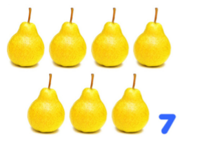
Рисунок 1.
«Натуральные числа» 👇
Определение 1
Натуральные числа (или естественные числа) — числа, которые возникают естественным образом при подсчете чего-либо.
Пример 1
Натуральными будут числа: $3, 48, 157, 1089, 25556$.
Если выстроить все натуральные числа в порядке их возрастания, то получим натуральный ряд.
Для определения натуральных чисел существует два подхода:
-
Числа, которые возникают при подсчете (нумерации) предметов (например, первый, второй и т.д.).
-
Числа, которые используют для обозначения количества предметов (нет стула, один стул, два стула и т.д.).
При первом подходе натуральный ряд начинается с единицы, при втором — с нуля.
Математики не пришли к единому выводу считать ли ноль натуральным числом. В большинстве российских источников традиционным является первый подход. Второй подход широко используется в программировании (например, при индексации массивов, нумерации битов машинного кода и т.д.).
Замечание 2
К натуральным числам не относятся ни отрицательные, ни нецелые числа.
Определение 2
Множество всех натуральных чисел обозначается $N=left{1, 2, 3, 4, dots , n, dots right}$ и характеризуется своей бесконечностью, т.к. для любого натурального числа $n$ существует натуральное число, которое будет большее $n$.
Пример 2
Какие из чисел являются натуральными?
[-6; 5; 0,6; frac{1}{2}; sqrt[3]{5}; 38; -38; 12,5; 4.]
Ответ: $5; 38; 4.$
При формулировке и доказательстве многих теорем арифметики натуральных чисел удобно использовать и ноль, поэтому при первом подходе применяется понятие расширенного множества натуральных чисел, которое содержит ноль и обозначается $N_0$ или $Z_0$.
Ноль как натуральное число
В русской литературе принято исключать нуль из числа натуральных чисел ($0notin N$), а множество натуральных чисел с нулём обозначают $N_0$.
В международной математической литературе множество $left{1, 2, 3, dots right}$ принято называть множеством положительных целых чисел и обозначать $Z+$. Множество $left{0, 1, 2, dots right}$ принято называть множеством неотрицательных целых чисел и обозначать $Z{ge 0}$.
Чтобы прочитать натуральное число, нужно выполнить следующие действия:
-
Разбить число справа налево на группы из $3$ цифр.
-
Прочитать слева направо по очереди группы из $3$ цифр и добавить название класса.
-
Название класса пропускают, если в группе цифр все нули.
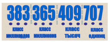
Рисунок 2.
Каждую цифру класса называют разрядом класса.
Меньшим натуральным числом является то, которое при проведении подсчета используется раньше. Например, число $9$ меньше $20$ (записывается $9 55$.
Аксиомы Пеано для натуральных чисел
Множество $N$ будем называть множеством натуральных чисел, если зафиксирован некоторый элемент единица $1in N$ и функция следования $S:Nto N$ так, что выполнены следующие условия:
-
$1in N$: единица является натуральным числом.
-
Если $xin N$, то $Sleft(xright)in N$: Если число — натуральное, то следующее число за ним тоже натуральное}.
-
$nexists xin N left(Sleft(xright)=1right)$: Не существует натурального числа, которое находится перед единицей}.
-
Если $Sleft(bright)=a$ и $Sleft(cright)=a$, тогда $b=c$: Если натуральное число $a$ следует за числом $b$ и за числом $c$, то $b=c$.
-
Аксиома индукции. Пусть $Pleft(nright)$ — некоторый одноместный предикат, который зависит от натурального числа $n$. Тогда:
Если $Pleft(1right)$ и $forall nleft(Pleft(nright)Longrightarrow Pleft(Sleft(nright)right)right)$, то $forall n Pleft(nright)$:
Если некоторое высказывание $P$ верно для $n=1$ и для любого $n$ из истинности $Pleft(nright)$ следует истинность $Pleft(n+1right)$, то $Pleft(nright)$ верно для любого натурального $n$.
Все аксиомы отражают представление о натуральном ряде и числовой линии.
Теоретико-множественное определение натуральных чисел (определение Фреге—Рассела)
По теории множеств единственным объектом конструирования любых математических систем является множество.
Таким образом, исходя из понятия множества натуральные числа вводятся по двум правилам:
- $0=emptyset $
-
$Sleft(nright)=ncup left{nright}$
-
Заданные таким образом числа называются порядковыми или ординальными.
Описываются первые порядковые числа и натуральные числа, которые им соответствуют, следующим образом:
-
$0=emptyset $
-
$1=left{0right}=left{emptyset right}$
-
$2=left{0, 1right}=left{emptyset , left{emptyset right}right}$
-
$3=left{0, 1, 2right}=left{emptyset , left{emptyset right}, left{emptyset , left{emptyset right}right}right}$
Находи статьи и создавай свой список литературы по ГОСТу
Поиск по теме
Натуральные числа
Определение. Натуральные числа — это числа, которые используются для счета: 1, 2, 3, …, n, …
Множество натуральных чисел принято обозначать символом N (от лат. naturalis — естественный).
Существуют два исторических подхода к определению натуральных чисел:
- это числа, возникающие при подсчёте (нумерации) предметов (первый, второй, третий, …);
- это числа, возникающие при обозначении количества предметов (нет предметов, один предмет, два предмета, …).
Натуральные числа в десятичной системе счисления записываются с помощью десяти цифр:
0, 1, 2, 3, 4, 5, 6, 7, 8, 9.
Множество натуральных чисел — является упорядоченным множеством, т.е. для любых натуральных чисел m и n справедливо одно из соотношений:
- либо m = n (m равно n),
- либо m > n (m больше n),
- либо m < n (m меньше n).
- Наименьшее натурально число — единица (1)
- Наибольшего натурального числа не существует.
- Нуль (0) не является натуральным числом.
Множество натуральных чисел бесконечно, так как для любого числа n всегда найдется число m, которое больше n
Из соседних натуральных чисел, число, которое стоит левее числа n называется предыдущим числу n, а число, которое стоит правее называется следующим за n.
Операции над натуральными числами
К замкнутым операциям над натуральными числами (операциям в результате, которых получается натуральных чисел) относятся следующие арифметические операции:
- Сложение
- Умножение
- Возведение в степень ab, где a — основание степени и b — показатель степени. Если основание и показатель — натуральные числа, то и результат будет являться натуральным числом.
Дополнительно рассматривают ещё две операции. С формальной точки зрения они не являются операциями над натуральными числами, так как их результат не всегда будет натуральным числом.
- Вычитание (При этом Уменьшаемое должно быть больше Вычитаемого)
- Деление
Классы и разряды
Разряд — положение (позиция) цифры в записи числа.
Низший разряд — самый правый. Старший разряд — самый левый.
Низший разряд — единицы, далее — десятки, сотни, тысячи, десятки тысяч, сотни тысяч, миллионы, десятки миллионов и т.д.
Пример:
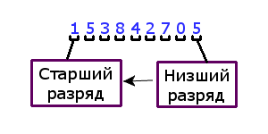
5 — единиц, 0 — десятков, 7 — сотен,
2 — тысячи, 4 — десятков тысяч, 8 — сотен тысяч,
3 — миллиона, 5 — десятков миллионов, 1 — сотня миллионов
Для удобства чтения, натуральных числа разбивают, на группы по три цифры в каждой начиная справа.
Класс — группа из трех цифр, на который разбито число, начиная справа. Последний класс может состоять из трех, двух или одной цифры.
- Первый класс — класс единиц;
- Второй класс — класс тысяч;
- Третий класс — класс миллионов;
- Четвертый класс — класс миллиардов;
- Пятый класс — класс триллионов;
- Шестой класс — класс квадрильонов (квадриллионов);
- Седьмой класс — класс квинтильонов (квинтиллионов);
- Восьмой класс — класс секстильонов;
- Девятый класс — класс септильонов;
Пример:
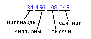
34 — миллиарда 456 миллионов 196 тысяч 45
Сравнение натуральных чисел
-
Сравнение натуральных чисел с разным количеством цифр
Среди натуральных чисел больше то, у которого больше цифр
-
Сравнение натуральных чисел с равным количеством цифр
Сравнить числа поразрядно, начиная со старшего разряда. Больше то, у которого больше единиц в наивысшем одноименном разряде
Пример:
3466 > 346 — так как число 3466 состоит из 4 цифр, а число 346 из 3 цифр.
34666 < 245784 — так как число 34666 состоит из 5 цифр, а число 245784 из 6 цифр.
Пример:
346 667 670 526 986
346 667 670 569 429
Второе из натуральных чисел с равным количеством цифр больше, так как 6 > 2.