Не следует путать с ʃ.
∫
Знак интеграла используется для обозначения интеграла в математике. Впервые он был использован немецким математиком и основателем дифференциального и интегрального исчислений Лейбницем в конце XVII века.
Символ (∫) образовался из буквы S (от лат. summa — сумма).
Юникод
| Знак | Unicode | Название | HTML-представление | LaTeX | |||
|---|---|---|---|---|---|---|---|
| Позиция | Название | Шестнадцатеричное | Десятичное | Мнемоника | |||
| ∫ | U+222B | Integral | Интеграл | ∫ | ∫ | ∫ | int |
| ∬ | U+222C | Double Integral | Двойной интеграл | ∬ | ∬ | iint | |
| ∭ | U+222D | Triple Integral | Тройной интеграл | ∭ | ∭ | iiint | |
| ∮ | U+222E | Contour Integral | Интеграл по контуру | ∮ | ∮ | oint | |
| ∯ | U+222F | Surface Integral | Интеграл по поверхности | ∯ | ∯ | oiint (требуется пакет esint) | |
| ∰ | U+2230 | Volume Integral | Интеграл по объёму | ∰ | ∰ | oiiint (требуется пакет esint) | |
| ∱ | U+2231 | Clockwise Integral | Интеграл с правым обходом | ∱ | ∱ | ||
| ∲ | U+2232 | Clockwise Contour Integral | Интеграл по контуру с правым обходом | ∲ | ∲ | ointclockwise (требуется пакет esint) | |
| ∳ | U+2233 | Anticlockwise Contour Integral | Интеграл по контуру с левым обходом | ∳ | ∳ | ointctrclockwise (требуется пакет esint) |
Традиции начертания
Русскоязычная традиция начертания знака интеграла отличается от принятой в некоторых западных странах.
-

В англоязычной традиции, реализованной в системе LaTeX, символ существенно наклонён вправо.
-

Немецкая форма интеграла вертикальна.
-

В русскоязычной литературе символ выглядит так.

См. также
- История математических обозначений
Ссылки
- Akademie Ausgabe Online (нем.)
- Полное собрание трудов (PDF)
- http://www.fileformat.info/info/unicode/char/222b/index.htm
Литература
- Александрова Н. В. История математических терминов, понятий, обозначений: Словарь-справочник. — СПб: ЛКИ, 2007. — 248 с.
Лучший ответ
Альона Марушкевич
Ученик
(198)
11 лет назад
В ворде щелкаете правой кнопкой мыши на панели инструментов и выбираете «Настройка». Затем заходите на вкладку «Команды» и выбираете пункт «Вставка», в поле справа ищете значок в виде корня квадратного из альфа, и вытаскиваете его на панель инструментов, после чего нажимая на него вы получите список всех математических знаков !!!
ИеговаМудрец (18606)
11 лет назад
«Редактор формул». Работает! Спасибо, научила!!))
Остальные ответы
Иегова
Мудрец
(18606)
11 лет назад
В Уорде меню вставка >> символ >> символы >> математические операторы >> ∫
Можно копировать мышью, можно задать на него комбинацию клавиш.
Кузьмич
Гуру
(3831)
11 лет назад
где? в какой программе?
Игорь ЗонаОракул (88613)
11 лет назад
блокнот
Кузьмич
Гуру
(3831)
вот там никак…
Alex
Профи
(979)
11 лет назад
Если ворд 2007, то вставка / функция
Анна Столярова
Профи
(787)
11 лет назад
вставка-объект-майкрософтэквишн3.0
Баян Сазамбаева
Ученик
(120)
6 лет назад
Где на клавиатуре знак интеграла или вставке?
Знак интеграла  используется для обозначения интеграла в математике. Впервые он был использован немецким философом, логиком, математиком, механиком, физиком, юристом, историком, дипломатом, изобретателем, языковедом и основателем дифференциального и интегрального исчислений Готфридом Вильгельмом Лейбницем (1646-1716) в конце 17 века.
Этот символ образовался из буквы S («длинная s»; от лат. ſumma (summa) – сумма).
Английский физик, математик, механик и астроном сэр Исаак Ньютон (1642-1727) в своих работах не предложил альтернативной символики интеграла, хотя пробовал различные варианты: вертикальную черту над функцией или символ квадрата, который стоит перед функцией или окаймляет её. Сам термин интеграл придумал швейцарский математик Якоб Бернулли (1654-1705) в 1690 году.
| Понравился сайт? Расскажи друзьям! | |
- Как правильно пишется слово «знак»
- Как правильно пишется слово «интеграл»
Делаем Карту слов лучше вместе

Привет! Меня зовут Лампобот, я компьютерная программа, которая помогает делать
Карту слов. Я отлично
умею считать, но пока плохо понимаю, как устроен ваш мир. Помоги мне разобраться!
Спасибо! Я обязательно научусь отличать широко распространённые слова от узкоспециальных.
Насколько понятно значение слова распаянный (прилагательное):
Ассоциации к слову «знак»
Ассоциации к слову «интеграл»
Синонимы к словосочетанию «знак интеграла»
Предложения со словосочетанием «знак интеграла»
- Знак интеграла симметричен относительно центра.
- Судороги изгибали тело знаком интеграла, желудок подскакивал к горлу и опускался вниз в ритм пульса, который, захлёбывался аритмией.
- (все предложения)
Значение словосочетания «знак интеграла»
-
Знак интеграла (∫) используется для обозначения интеграла в математике. Впервые он был использован немецким математиком и одним из основателей дифференциального и интегрального исчислений Лейбницем в конце XVII века. (Википедия)
Все значения словосочетания ЗНАК ИНТЕГРАЛА
Афоризмы русских писателей со словом «знак»
- Знаки препинания, служащие нотами при чтении, расставлены… как пуговицы на мундире гоголевского городничего.
- Еще Пушкин говорил о знаках препинания. Они существуют, чтобы выделить мысль, привести слова в правильное соотношение и дать фразе легкость и правильное звучание. Знаки препинания — это как нотные знаки. Они твердо держат текст и не дают ему рассыпаться.
- В художественном произведении знаки препинания зачастую играют роль нот, и выучиться им по учебнику нельзя: нужны еще чутье и опыт.
- (все афоризмы русских писателей)
![]()
sergeewitch
24 декабря 2021
Не следует путать с ʃ.
∫
Знак интеграла используется для обозначения интеграла в математике. Впервые он был использован немецким математиком и основателем дифференциального и интегрального исчислений Лейбницем в конце XVII века.
Символ (∫) образовался из буквы S (от лат. summa — сумма).
Юникод
| Знак | Unicode | Название | HTML-представление | LaTeX | |||
|---|---|---|---|---|---|---|---|
| Позиция | Название | Шестнадцатеричное | Десятичное | Мнемоника | |||
| ∫ | U+222B | Integral | Интеграл | ∫ | ∫ | ∫ | int |
| ∬ | U+222C | Double Integral | Двойной интеграл | ∬ | ∬ | iint | |
| ∭ | U+222D | Triple Integral | Тройной интеграл | ∭ | ∭ | iiint | |
| ∮ | U+222E | Contour Integral | Интеграл по контуру | ∮ | ∮ | oint | |
| ∯ | U+222F | Surface Integral | Интеграл по поверхности | ∯ | ∯ | oiint (требуется пакет esint) | |
| ∰ | U+2230 | Volume Integral | Интеграл по объёму | ∰ | ∰ | oiiint (требуется пакет esint) | |
| ∱ | U+2231 | Clockwise Integral | Интеграл с правым обходом | ∱ | ∱ | ||
| ∲ | U+2232 | Clockwise Contour Integral | Интеграл по контуру с правым обходом | ∲ | ∲ | ointclockwise (требуется пакет esint) | |
| ∳ | U+2233 | Anticlockwise Contour Integral | Интеграл по контуру с левым обходом | ∳ | ∳ | ointctrclockwise (требуется пакет esint) |
Традиции начертания
Русскоязычная традиция начертания знака интеграла отличается от принятой в некоторых западных странах.
-
В англоязычной традиции, реализованной в системе LaTeX, символ существенно наклонён вправо.
-
Немецкая форма интеграла вертикальна.
-
В русскоязычной литературе символ выглядит так.
См. также
- История математических обозначений
| |
|---|
| Плюс ( + ) • Минус ( − ) • Знак умножения ( · или × ) • Знак деления ( : или / ) • Знак корня ( √ ) • Знак равенства ( =, ≈, ≡ и др.) • Знаки неравенства ( ≠, >, < и др.) • Бесконечность ( ∞ ) • Знак интеграла ( ∫ ) • Факториал ( ! ) • Вертикальная черта ( | ) • Знак градуса ( ° ) • Минута градуса ( ′ ) • Секунда градуса ( ″ ) • Штрих ( ′ ) • Звёздочка ( * ) • Обратная косая черта, бэкслеш ( ) • Процент ( % ) • Промилле ( ‰ ) • Тильда ( ~ ) • Циркумфлекс ( ^ ) • Плюс-минус ( ± ) • Обелюс ( ÷ ) • Десятичный разделитель ( , или . ) |
| Математика • История математических обозначений |
Ссылки
- Akademie Ausgabe Online (нем.)
- Полное собрание трудов (PDF)
- http://www.fileformat.info/info/unicode/char/222b/index.htm
Литература
- Александрова Н. В. История математических терминов, понятий, обозначений: Словарь-справочник. — СПб: ЛКИ, 2007. — 248 с.
Интеграл — это математическая функция, используемая в исчислении. Вы можете вводить интегральные уравнения в документы Office с помощью редактора формул. Однако, когда вам просто нужно ввести целые символы, легко использовать сочетания клавиш. В отличие от редактора формул, сочетания клавиш помогают вводить символы, как обычные текстовые символы, выровненные с другим содержимым документа.
Связанный: Сочетания клавиш Alt-кода для математических символов.
Сочетания клавиш для встроенных символов
Ниже приведены различные интегральные символы, доступные в Unicode как часть символов математического оператора между кодовыми точками 2200–22FF.
| Условное обозначение | название | Код Windows | Код Mac |
|---|---|---|---|
| ∫ | интеграл | Alt + 8747 | Вариант + 222B |
| ∬ | Двойной интеграл | Alt + 8748 | Вариант + 222C |
| ∭ | Тройной интеграл | Alt + 8749 | Вариант + 222D |
| ∮ | Contour Integral | Alt + 8750 | Option + 222E |
| ∯ | Поверхностный интеграл | Alt + 8751 | Вариант + 222F |
| ∰ | Объемный интеграл | Alt + 8752 | Вариант + 2230 |
| ∱ | Интеграл по часовой стрелке | Alt + 8753 | Вариант + 2231 |
| ∲ | Контурный интеграл по часовой стрелке | Alt + 8754 | Вариант + 2232 |
| ∳ | Контурный интеграл против часовой стрелки | Alt + 8755 | Вариант + 2233 |
| ⌠ | Верхняя половина Integral | Alt + 8992 | Вариант + 2320 |
| ⌡ | Нижняя половина интегрального | Alt + 8993 | Вариант + 2321 |
| ⎮ | Интегральное расширение | Alt + 9134 | Вариант + 23AE |
| ⨋ | Суммирование с интегралом | Alt + 10763 | Вариант + 2A0B |
| ⨌ | Четверной интегральный оператор | Alt + 10764 | Вариант + 2A0C |
| ⨍ | Конечная часть интеграла | Alt + 10765 | Вариант + 2A0D |
| ⨎ | Интегральный с двойным ходом | Alt + 10766 | Вариант + 2A0E |
| ⨏ | Интегральное среднее с косой чертой | Alt + 10767 | Option + 2A0F |
| ⨕ | Интеграл вокруг точечного оператора | Alt + 10773 | Вариант + 2A15 |
| ⨖ | Кватернионный интегральный оператор | Alt + 10774 | Вариант + 2A16 |
| ⨗ | Интегральный со стрелкой влево с крючком | Alt + 10775 | Вариант + 2A17 |
| ⨘ | Интеграл со знаком времени | Alt + 10776 | Вариант + 2A18 |
| ⨙ | Интеграл с пересечением | Alt + 10777 | Вариант + 2A19 |
| ⨚ | Интеграл с Union | Alt + 10778 | Вариант + 2A1A |
| ⨛ | Интеграл с Overbar | Alt + 10779 | Вариант + 2A1B |
| ⨜ | Интегрально с нижней панелью | Alt + 10780 | Option + 2A1C |
Как набирать интегральные символы?
1. Введите целые символы в Windows.
Если вы хотите вставить интегральные символы в документы на базе Windows, используйте ярлыки альтернативного кода, указанные в столбце «Код Windows» в приведенной выше таблице. Например, alt + 10776 сделает интеграл со знаком времени как.
2. Ярлык для документов Word.
В документе Microsoft Word вы можете использовать шестнадцатеричный код, указанный в последнем столбце приведенной выше таблицы. Например, 2A19 Alt + X составит интеграл с символом пересечения, например ⨙.
3. Ввод целых символов в Mac
Если у вас Mac, используйте «Код Mac», указанный в таблице выше. Например, option + 2A1C будет составлять интеграл с символом подчеркивания, например ⨜.
Примечание: Первый метод альтернативных кодов будет работать только с цифровой клавиатурой, поэтому вы можете использовать второй метод, используя обычные цифровые клавиши клавиатуры. Для третьего метода на Mac вам необходимо изменить метод ввода языка на Unicode Hex Input и переключить ввод из верхней панели меню.
Пример HTML-кода
Если вы хотите вставить интегральные символы в HTML, используйте один из форматов, приведенных в приведенном ниже примере кода. Обратите внимание, что только интегральный символ ∫ имеет имя объекта & int; и использовать десятичные и шестнадцатеричные коды для других символов в данном формате.
<span>∫</span>
<span>∫</span>
<span>∫</span>Пример кода CSS
Подобно HTML, вы также можете вставлять символы в CSS, используя шестнадцатеричный код. Ниже приведен пример кода, и вы можете использовать любое семейство шрифтов в коде.
li:before {
	content:222B;
	font-family:Arial;
}
Помните, как уже упоминалось, для математической документации вам следует использовать редактор формул или программное обеспечение, такое как LaTeX. В документах Office выберите «Вставить> Уравнение», чтобы открыть редактор формул. Щелкните раскрывающийся список «Интегральный», чтобы получить различные символы интеграла и создать уравнения.
Решение интегралов – задача легкая, но только для избранных. Эта статья для тех, кто хочет научиться понимать интегралы, но не знает о них ничего или почти ничего. Интеграл… Зачем он нужен? Как его вычислять? Что такое определенный и неопределенный интегралы?
Если единственное известное вам применение интеграла – доставать крючком в форме значка интеграла что-то полезное из труднодоступных мест, тогда добро пожаловать! Узнайте, как решать простейшие и другие интегралы и почему без этого никак нельзя обойтись в математике.
Ежедневная рассылка с полезной информацией для студентов всех направлений – на нашем телеграм-канале.
Изучаем понятие «интеграл»
Интегрирование было известно еще в Древнем Египте. Конечно, не в современном виде, но все же. С тех пор математики написали очень много книг по этой теме. Особенно отличились Ньютон и Лейбниц, но суть вещей не изменилась.
Как понять интегралы с нуля? Никак! Для понимания этой темы все равно понадобятся базовые знания основ математического анализа. Сведения о пределах и производных, необходимые и для понимания интегралов, уже есть у нас в блоге.
Неопределенный интеграл
Пусть у нас есть какая-то функция f(x).
Неопределенным интегралом функции f(x) называется такая функция F(x), производная которой равна функции f(x).
Другими словами интеграл – это производная наоборот или первообразная. Кстати, о том, как вычислять производные, читайте в нашей статье.

Первообразная существует для всех непрерывных функций. Также к первообразной часто прибавляют знак константы, так как производные функций, различающихся на константу, совпадают. Процесс нахождения интеграла называется интегрированием.
Простой пример:
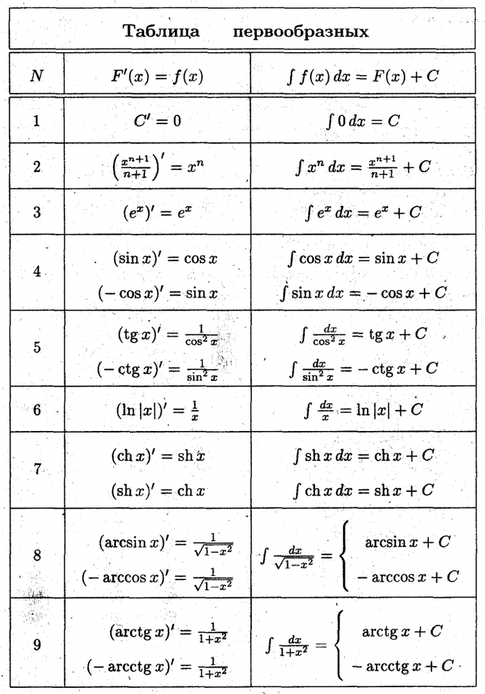
Чтобы постоянно не высчитывать первообразные элементарных функций, их удобно свести в таблицу и пользоваться уже готовыми значениями.
Полная таблица интегралов для студентов
Определенный интеграл
Имея дело с понятием интеграла, мы имеем дело с бесконечно малыми величинами. Интеграл поможет вычислить площадь фигуры, массу неоднородного тела, пройденный при неравномерном движении путь и многое другое. Следует помнить, что интеграл – это сумма бесконечно большого количества бесконечно малых слагаемых.
В качестве примера представим себе график какой-нибудь функции.
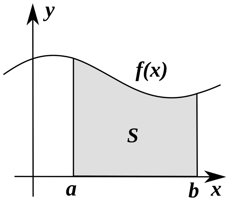
Как найти площадь фигуры, ограниченной графиком функции? С помощью интеграла! Разобьем криволинейную трапецию, ограниченную осями координат и графиком функции, на бесконечно малые отрезки. Таким образом фигура окажется разделена на тонкие столбики. Сумма площадей столбиков и будет составлять площадь трапеции. Но помните, что такое вычисление даст примерный результат. Однако чем меньше и уже будут отрезки, тем точнее будет вычисление. Если мы уменьшим их до такой степени, что длина будет стремиться к нулю, то сумма площадей отрезков будет стремиться к площади фигуры. Это и есть определенный интеграл, который записывается так:
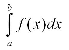
Точки а и b называются пределами интегрирования.

«Интеграл»
Кстати! Для наших читателей сейчас действует скидка 10% на любой вид работы
Правила вычисления интегралов для чайников
Свойства неопределенного интеграла
Как решить неопределенный интеграл? Здесь мы рассмотрим свойства неопределенного интеграла, которые пригодятся при решении примеров.
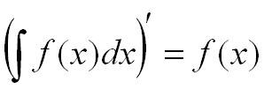
- Производная от интеграла равна подынтегральной функции:
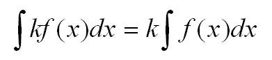
- Константу можно выносить из-под знака интеграла:
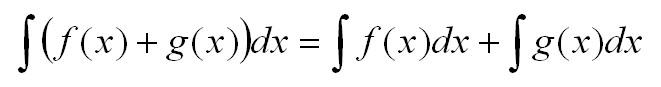
- Интеграл от суммы равен сумме интегралов. Верно также для разности:
Свойства определенного интеграла
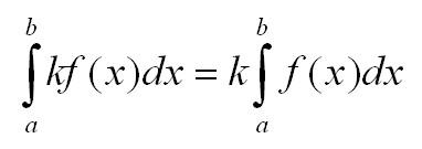
- Линейность:
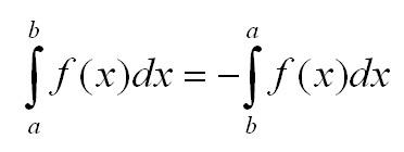
- Знак интеграла изменяется, если поменять местами пределы интегрирования:
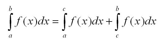
- При любых точках a, b и с:
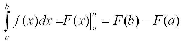
Как считать определенный интеграл? С помощью формулы Ньютона-Лейбница.
Мы уже выяснили, что определенный интеграл – это предел суммы. Но как получить конкретное значение при решении примера? Для этого существует формула Ньютона-Лейбница:
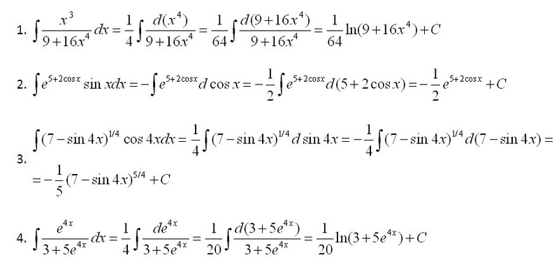
Примеры решения интегралов
Ниже рассмотрим неопределенный интеграл и примеры с решением. Предлагаем самостоятельно разобраться в тонкостях решения, а если что-то непонятно, задавайте вопросы в комментариях.
Для закрепления материала посмотрите видео о том, как решаются интегралы на практике. Не отчаиваетесь, если интеграл не дается сразу. Обратитесь в профессиональный сервис для студентов, и любой тройной или криволинейный интеграл по замкнутой поверхности станет вам по силам.

Иван Колобков, известный также как Джони. Маркетолог, аналитик и копирайтер компании Zaochnik. Подающий надежды молодой писатель. Питает любовь к физике, раритетным вещам и творчеству Ч. Буковски.
Знак интеграла
∫
Знак интеграла (∫) используется для обозначения интеграла в математике. Впервые он был использован немецким математиком и одним из основателей дифференциального и интегрального исчислений Лейбницем в конце XVII века.
Символ «∫» образовался из буквы ſ («длинная s»; от лат. ſumma (summa) — сумма)[1].
Юникод
| Знак | Юникод | Название | HTML-представление | LaTeX | |||
|---|---|---|---|---|---|---|---|
| Позиция | Название | Шестнадцатеричное | Десятичное | Мнемоника | |||
| ∫ | U+222B | integral | Интеграл | ∫ | ∫ | ∫ | int |
| ∬ | U+222C | double integral | Двойной интеграл | ∬ | ∬ | iint | |
| ∭ | U+222D | triple integral | Тройной интеграл | ∭ | ∭ | iiint | |
| ∮ | U+222E | contour integral | Интеграл по контуру | ∮ | ∮ | oint | |
| ∯ | U+222F | surface integral | Интеграл по поверхности | ∯ | ∯ | oiint (требуется пакет esint) | |
| ∰ | U+2230 | volume integral | Интеграл по объёму | ∰ | ∰ | oiiint (требуется пакет esint) | |
| ∱ | U+2231 | clockwise integral | Интеграл с правым обходом | ∱ | ∱ | ||
| ∲ | U+2232 | clockwise contour integral | Интеграл по контуру с правым обходом | ∲ | ∲ | ointclockwise (требуется пакет esint) | |
| ∳ | U+2233 | anticlockwise contour integral | Интеграл по контуру с левым обходом | ∳ | ∳ | ointctrclockwise (требуется пакет esint) |
Традиции начертания
Русскоязычная традиция начертания знака интеграла отличается от принятой в некоторых западных странах.
-
В англоязычной традиции, реализованной в системе LaTeX, символ существенно наклонён вправо.
-
Немецкая форма интеграла вертикальна.
-
В русскоязычной литературе символ выглядит так.


Примечания
- ↑
Florian Cajori. A history of mathematical notations. — Courier Dover Publications, 1993. — P. 203. — 818 p. — (Dover books on mathematics). — ISBN 9780486677668.
См. также
- История математических обозначений
Литература
- Александрова Н. В. История математических терминов, понятий, обозначений: Словарь-справочник. — СПб: ЛКИ, 2007. — 248 с.
Ссылки
- Akademie Ausgabe Online (нем.)
- Полное собрание трудов (PDF)
- http://www.fileformat.info/info/unicode/char/222b/index.htm
Математические знаки |
|---|
|
|
This article is about the concept of definite integrals in calculus. For the indefinite integral, see antiderivative. For the set of numbers, see integer. For other uses, see Integral (disambiguation).
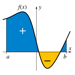
A definite integral of a function can be represented as the signed area of the region bounded by its graph. In the above graph as an example, the integral of  is the blue (+) area subtracted by the yellow (-) area.
In mathematics, an integral assigns numbers to functions in a way that describes displacement, area, volume, and other concepts that arise by combining infinitesimal data. The process of finding integrals is called integration. Along with differentiation, integration is a fundamental, essential operation of calculus,[a] and serves as a tool to solve problems in mathematics and physics involving the area of an arbitrary shape, the length of a curve, and the volume of a solid, among others.
The integrals enumerated here are those termed definite integrals, which can be interpreted as the signed area of the region in the plane that is bounded by the graph of a given function between two points in the real line. Conventionally, areas above the horizontal axis of the plane are positive while areas below are negative. Integrals also refer to the concept of an antiderivative, a function whose derivative is the given function. In this case, they are called indefinite integrals. The fundamental theorem of calculus relates definite integrals with differentiation and provides a method to compute the definite integral of a function when its antiderivative is known.
Although methods of calculating areas and volumes dated from ancient Greek mathematics, the principles of integration were formulated independently by Isaac Newton and Gottfried Wilhelm Leibniz in the late 17th century, who thought of the area under a curve as an infinite sum of rectangles of infinitesimal width. Bernhard Riemann later gave a rigorous definition of integrals, which is based on a limiting procedure that approximates the area of a curvilinear region by breaking the region into infinitesimally thin vertical slabs. In the early 20th century, Henri Lebesgue generalized Riemann’s formulation by introducing what is now referred to as the Lebesgue integral; it is more robust than Riemann’s in the sense that a wider class of functions are Lebesgue-integrable.
Integrals may be generalized depending on the type of the function as well as the domain over which the integration is performed. For example, a line integral is defined for functions of two or more variables, and the interval of integration is replaced by a curve connecting the two endpoints of the interval. In a surface integral, the curve is replaced by a piece of a surface in three-dimensional space.
History[edit]
Pre-calculus integration[edit]
The first documented systematic technique capable of determining integrals is the method of exhaustion of the ancient Greek astronomer Eudoxus (ca. 370 BC), which sought to find areas and volumes by breaking them up into an infinite number of divisions for which the area or volume was known.[1] This method was further developed and employed by Archimedes in the 3rd century BC and used to calculate the area of a circle, the surface area and volume of a sphere, area of an ellipse, the area under a parabola, the volume of a segment of a paraboloid of revolution, the volume of a segment of a hyperboloid of revolution, and the area of a spiral.[2]
A similar method was independently developed in China around the 3rd century AD by Liu Hui, who used it to find the area of the circle. This method was later used in the 5th century by Chinese father-and-son mathematicians Zu Chongzhi and Zu Geng to find the volume of a sphere.[3]
In the Middle East, Hasan Ibn al-Haytham, Latinized as Alhazen (c. 965 – c. 1040 AD) derived a formula for the sum of fourth powers.[4] He used the results to carry out what would now be called an integration of this function, where the formulae for the sums of integral squares and fourth powers allowed him to calculate the volume of a paraboloid.[5]
The next significant advances in integral calculus did not begin to appear until the 17th century. At this time, the work of Cavalieri with his method of Indivisibles, and work by Fermat, began to lay the foundations of modern calculus,[6] with Cavalieri computing the integrals of xn up to degree n = 9 in Cavalieri’s quadrature formula.[7] The case n = −1 required the invention of a function, hyperbolic logarithm, achieved by quadrature of the hyperbola in 1647.
Further steps were made in the early 17th century by Barrow and Torricelli, who provided the first hints of a connection between integration and differentiation. Barrow provided the first proof of the fundamental theorem of calculus.[8] Wallis generalized Cavalieri’s method, computing integrals of x to a general power, including negative powers and fractional powers.[9]
Leibniz and Newton[edit]
The major advance in integration came in the 17th century with the independent discovery of the fundamental theorem of calculus by Leibniz and Newton.[10] The theorem demonstrates a connection between integration and differentiation. This connection, combined with the comparative ease of differentiation, can be exploited to calculate integrals. In particular, the fundamental theorem of calculus allows one to solve a much broader class of problems. Equal in importance is the comprehensive mathematical framework that both Leibniz and Newton developed. Given the name infinitesimal calculus, it allowed for precise analysis of functions within continuous domains. This framework eventually became modern calculus, whose notation for integrals is drawn directly from the work of Leibniz.
Formalization[edit]
While Newton and Leibniz provided a systematic approach to integration, their work lacked a degree of rigour. Bishop Berkeley memorably attacked the vanishing increments used by Newton, calling them «ghosts of departed quantities».[11] Calculus acquired a firmer footing with the development of limits. Integration was first rigorously formalized, using limits, by Riemann.[12] Although all bounded piecewise continuous functions are Riemann-integrable on a bounded interval, subsequently more general functions were considered—particularly in the context of Fourier analysis—to which Riemann’s definition does not apply, and Lebesgue formulated a different definition of integral, founded in measure theory (a subfield of real analysis). Other definitions of integral, extending Riemann’s and Lebesgue’s approaches, were proposed. These approaches based on the real number system are the ones most common today, but alternative approaches exist, such as a definition of integral as the standard part of an infinite Riemann sum, based on the hyperreal number system.
Historical notation[edit]
The notation for the indefinite integral was introduced by Gottfried Wilhelm Leibniz in 1675.[13] He adapted the integral symbol, ∫, from the letter ſ (long s), standing for summa (written as ſumma; Latin for «sum» or «total»). The modern notation for the definite integral, with limits above and below the integral sign, was first used by Joseph Fourier in Mémoires of the French Academy around 1819–20, reprinted in his book of 1822.[14]
Isaac Newton used a small vertical bar above a variable to indicate integration, or placed the variable inside a box. The vertical bar was easily confused with .x or x′, which are used to indicate differentiation, and the box notation was difficult for printers to reproduce, so these notations were not widely adopted.[15]
First use of the term[edit]
The term was first printed in Latin by Jacob Bernoulli in 1690: «Ergo et horum Integralia aequantur».[16]
Terminology and notation[edit]
In general, the integral of a real-valued function f(x) with respect to a real variable x on an interval [a, b] is written as

The integral sign ∫ represents integration. The symbol dx, called the differential of the variable x, indicates that the variable of integration is x. The function f(x) is called the integrand, the points a and b are called the limits (or bounds) of integration, and the integral is said to be over the interval [a, b], called the interval of integration.[17]
A function is said to be integrable if its integral over its domain is finite. If limits are specified, the integral is called a definite integral.
When the limits are omitted, as in

the integral is called an indefinite integral, which represents a class of functions (the antiderivative) whose derivative is the integrand.[18] The fundamental theorem of calculus relates the evaluation of definite integrals to indefinite integrals. There are several extensions of the notation for integrals to encompass integration on unbounded domains and/or in multiple dimensions (see later sections of this article).
In advanced settings, it is not uncommon to leave out dx when only the simple Riemann integral is being used, or the exact type of integral is immaterial. For instance, one might write  to express the linearity of the integral, a property shared by the Riemann integral and all generalizations thereof.[19]
Interpretations[edit]
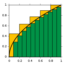
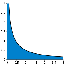
Approximations to integral of √x from 0 to 1, with 5 yellow right endpoint partitions and 12 green left endpoint partitions
Integrals appear in many practical situations. For instance, from the length, width and depth of a swimming pool which is rectangular with a flat bottom, one can determine the volume of water it can contain, the area of its surface, and the length of its edge. But if it is oval with a rounded bottom, integrals are required to find exact and rigorous values for these quantities. In each case, one may divide the sought quantity into infinitely many infinitesimal pieces, then sum the pieces to achieve an accurate approximation.
For example, to find the area of the region bounded by the graph of the function f(x) = √x between x = 0 and x = 1, one can cross the interval in five steps (0, 1/5, 2/5, …, 1), then fill a rectangle using the right end height of each piece (thus √0, √1/5, √2/5, …, √1) and sum their areas to get an approximation of

which is larger than the exact value. Alternatively, when replacing these subintervals by ones with the left end height of each piece, the approximation one gets is too low: with twelve such subintervals the approximated area is only 0.6203. However, when the number of pieces increase to infinity, it will reach a limit which is the exact value of the area sought (in this case, 2/3). One writes

which means 2/3 is the result of a weighted sum of function values, √x, multiplied by the infinitesimal step widths, denoted by dx, on the interval [0, 1].
Darboux upper sums of the function y = x2

Darboux lower sums of the function y = x2
Formal definitions[edit]

Riemann sums converging
There are many ways of formally defining an integral, not all of which are equivalent. The differences exist mostly to deal with differing special cases which may not be integrable under other definitions, but also occasionally for pedagogical reasons. The most commonly used definitions are Riemann integrals and Lebesgue integrals.
Riemann integral[edit]
The Riemann integral is defined in terms of Riemann sums of functions with respect to tagged partitions of an interval.[20] A tagged partition of a closed interval [a, b] on the real line is a finite sequence

This partitions the interval [a, b] into n sub-intervals [xi−1, xi] indexed by i, each of which is «tagged» with a distinguished point ti ∈ [xi−1, xi]. A Riemann sum of a function f with respect to such a tagged partition is defined as

thus each term of the sum is the area of a rectangle with height equal to the function value at the distinguished point of the given sub-interval, and width the same as the width of sub-interval, Δi = xi−xi−1. The mesh of such a tagged partition is the width of the largest sub-interval formed by the partition, maxi=1…n Δi. The Riemann integral of a function f over the interval [a, b] is equal to S if:[21]
- For all
 there exists such that, for any tagged partition with mesh less than ,


When the chosen tags give the maximum (respectively, minimum) value of each interval, the Riemann sum becomes an upper (respectively, lower) Darboux sum, suggesting the close connection between the Riemann integral and the Darboux integral.
Lebesgue integral[edit]
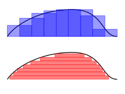
Riemann–Darboux’s integration (top) and Lebesgue integration (bottom)
It is often of interest, both in theory and applications, to be able to pass to the limit under the integral. For instance, a sequence of functions can frequently be constructed that approximate, in a suitable sense, the solution to a problem. Then the integral of the solution function should be the limit of the integrals of the approximations. However, many functions that can be obtained as limits are not Riemann-integrable, and so such limit theorems do not hold with the Riemann integral. Therefore, it is of great importance to have a definition of the integral that allows a wider class of functions to be integrated.[22]
Such an integral is the Lebesgue integral, that exploits the following fact to enlarge the class of integrable functions: if the values of a function are rearranged over the domain, the integral of a function should remain the same. Thus Henri Lebesgue introduced the integral bearing his name, explaining this integral thus in a letter to Paul Montel:[23]
I have to pay a certain sum, which I have collected in my pocket. I take the bills and coins out of my pocket and give them to the creditor in the order I find them until I have reached the total sum. This is the Riemann integral. But I can proceed differently. After I have taken all the money out of my pocket I order the bills and coins according to identical values and then I pay the several heaps one after the other to the creditor. This is my integral.
As Folland puts it, «To compute the Riemann integral of f, one partitions the domain [a, b] into subintervals», while in the Lebesgue integral, «one is in effect partitioning the range of f «.[24] The definition of the Lebesgue integral thus begins with a measure, μ. In the simplest case, the Lebesgue measure μ(A) of an interval A = [a, b] is its width, b − a, so that the Lebesgue integral agrees with the (proper) Riemann integral when both exist.[25] In more complicated cases, the sets being measured can be highly fragmented, with no continuity and no resemblance to intervals.
Using the «partitioning the range of f » philosophy, the integral of a non-negative function f : R → R should be the sum over t of the areas between a thin horizontal strip between y = t and y = t + dt. This area is just μ{ x : f(x) > t} dt. Let f∗(t) = μ{ x : f(x) > t }. The Lebesgue integral of f is then defined by

where the integral on the right is an ordinary improper Riemann integral (f∗ is a strictly decreasing positive function, and therefore has a well-defined improper Riemann integral).[26] For a suitable class of functions (the measurable functions) this defines the Lebesgue integral.
A general measurable function f is Lebesgue-integrable if the sum of the absolute values of the areas of the regions between the graph of f and the x-axis is finite:[27]

In that case, the integral is, as in the Riemannian case, the difference between the area above the x-axis and the area below the x-axis:[28]

where

Other integrals[edit]
Although the Riemann and Lebesgue integrals are the most widely used definitions of the integral, a number of others exist, including:
- The Darboux integral, which is defined by Darboux sums (restricted Riemann sums) yet is equivalent to the Riemann integral. A function is Darboux-integrable if and only if it is Riemann-integrable. Darboux integrals have the advantage of being easier to define than Riemann integrals.
- The Riemann–Stieltjes integral, an extension of the Riemann integral which integrates with respect to a function as opposed to a variable.
- The Lebesgue–Stieltjes integral, further developed by Johann Radon, which generalizes both the Riemann–Stieltjes and Lebesgue integrals.
- The Daniell integral, which subsumes the Lebesgue integral and Lebesgue–Stieltjes integral without depending on measures.
- The Haar integral, used for integration on locally compact topological groups, introduced by Alfréd Haar in 1933.
- The Henstock–Kurzweil integral, variously defined by Arnaud Denjoy, Oskar Perron, and (most elegantly, as the gauge integral) Jaroslav Kurzweil, and developed by Ralph Henstock.
- The Itô integral and Stratonovich integral, which define integration with respect to semimartingales such as Brownian motion.
- The Young integral, which is a kind of Riemann–Stieltjes integral with respect to certain functions of unbounded variation.
- The rough path integral, which is defined for functions equipped with some additional «rough path» structure and generalizes stochastic integration against both semimartingales and processes such as the fractional Brownian motion.
- The Choquet integral, a subadditive or superadditive integral created by the French mathematician Gustave Choquet in 1953.
- The Bochner integral, an extension of the Lebesgue integral to a more general class of functions, namely, those with a domain that is a Banach space.
Properties[edit]
Linearity[edit]
The collection of Riemann-integrable functions on a closed interval [a, b] forms a vector space under the operations of pointwise addition and multiplication by a scalar, and the operation of integration

is a linear functional on this vector space. Thus, the collection of integrable functions is closed under taking linear combinations, and the integral of a linear combination is the linear combination of the integrals:[29]

Similarly, the set of real-valued Lebesgue-integrable functions on a given measure space E with measure μ is closed under taking linear combinations and hence form a vector space, and the Lebesgue integral

is a linear functional on this vector space, so that:[28]

More generally, consider the vector space of all measurable functions on a measure space (E,μ), taking values in a locally compact complete topological vector space V over a locally compact topological field K, f : E → V. Then one may define an abstract integration map assigning to each function f an element of V or the symbol ∞,

that is compatible with linear combinations.[30] In this situation, the linearity holds for the subspace of functions whose integral is an element of V (i.e. «finite»). The most important special cases arise when K is R, C, or a finite extension of the field Qp of p-adic numbers, and V is a finite-dimensional vector space over K, and when K = C and V is a complex Hilbert space.
Linearity, together with some natural continuity properties and normalization for a certain class of «simple» functions, may be used to give an alternative definition of the integral. This is the approach of Daniell for the case of real-valued functions on a set X, generalized by Nicolas Bourbaki to functions with values in a locally compact topological vector space. See Hildebrandt 1953 for an axiomatic characterization of the integral.
Inequalities[edit]
A number of general inequalities hold for Riemann-integrable functions defined on a closed and bounded interval [a, b] and can be generalized to other notions of integral (Lebesgue and Daniell).
- Upper and lower bounds. An integrable function f on [a, b], is necessarily bounded on that interval. Thus there are real numbers m and M so that m ≤ f (x) ≤ M for all x in [a, b]. Since the lower and upper sums of f over [a, b] are therefore bounded by, respectively, m(b − a) and M(b − a), it follows that
- Inequalities between functions.[31] If f(x) ≤ g(x) for each x in [a, b] then each of the upper and lower sums of f is bounded above by the upper and lower sums, respectively, of g. Thus
This is a generalization of the above inequalities, as M(b − a) is the integral of the constant function with value M over [a, b]. In addition, if the inequality between functions is strict, then the inequality between integrals is also strict. That is, if f(x) < g(x) for each x in [a, b], then
- Subintervals. If [c, d] is a subinterval of [a, b] and f (x) is non-negative for all x, then
- Products and absolute values of functions. If f and g are two functions, then we may consider their pointwise products and powers, and absolute values:
If f is Riemann-integrable on [a, b] then the same is true for |f|, and
Moreover, if f and g are both Riemann-integrable then fg is also Riemann-integrable, and
This inequality, known as the Cauchy–Schwarz inequality, plays a prominent role in Hilbert space theory, where the left hand side is interpreted as the inner product of two square-integrable functions f and g on the interval [a, b].
- Hölder’s inequality.[32] Suppose that p and q are two real numbers, 1 ≤ p, q ≤ ∞ with 1/p + 1/q = 1, and f and g are two Riemann-integrable functions. Then the functions |f|p and |g|q are also integrable and the following Hölder’s inequality holds:
For p = q = 2, Hölder’s inequality becomes the Cauchy–Schwarz inequality.
- Minkowski inequality.[32] Suppose that p ≥ 1 is a real number and f and g are Riemann-integrable functions. Then | f |p, | g |p and | f + g |p are also Riemann-integrable and the following Minkowski inequality holds:
An analogue of this inequality for Lebesgue integral is used in construction of Lp spaces.


Conventions[edit]
In this section, f is a real-valued Riemann-integrable function. The integral

over an interval [a, b] is defined if a < b. This means that the upper and lower sums of the function f are evaluated on a partition a = x0 ≤ x1 ≤ . . . ≤ xn = b whose values xi are increasing. Geometrically, this signifies that integration takes place «left to right», evaluating f within intervals [x i , x i +1] where an interval with a higher index lies to the right of one with a lower index. The values a and b, the end-points of the interval, are called the limits of integration of f. Integrals can also be defined if a > b:[17]

With a = b, this implies:

The first convention is necessary in consideration of taking integrals over subintervals of [a, b]; the second says that an integral taken over a degenerate interval, or a point, should be zero. One reason for the first convention is that the integrability of f on an interval [a, b] implies that f is integrable on any subinterval [c, d], but in particular integrals have the property that if c is any element of [a, b], then:[29]

With the first convention, the resulting relation

is then well-defined for any cyclic permutation of a, b, and c.
Fundamental theorem of calculus[edit]
The fundamental theorem of calculus is the statement that differentiation and integration are inverse operations: if a continuous function is first integrated and then differentiated, the original function is retrieved.[33] An important consequence, sometimes called the second fundamental theorem of calculus, allows one to compute integrals by using an antiderivative of the function to be integrated.[34]
First theorem[edit]
Let f be a continuous real-valued function defined on a closed interval [a, b]. Let F be the function defined, for all x in [a, b], by

Then, F is continuous on [a, b], differentiable on the open interval (a, b), and

for all x in (a, b).
Second theorem[edit]
Let f be a real-valued function defined on a closed interval [a, b] that admits an antiderivative F on [a, b]. That is, f and F are functions such that for all x in [a, b],

If f is integrable on [a, b] then

Extensions[edit]
Improper integrals[edit]
A «proper» Riemann integral assumes the integrand is defined and finite on a closed and bounded interval, bracketed by the limits of integration. An improper integral occurs when one or more of these conditions is not satisfied. In some cases such integrals may be defined by considering the limit of a sequence of proper Riemann integrals on progressively larger intervals.
If the interval is unbounded, for instance at its upper end, then the improper integral is the limit as that endpoint goes to infinity:[35]

If the integrand is only defined or finite on a half-open interval, for instance (a, b], then again a limit may provide a finite result:[36]

That is, the improper integral is the limit of proper integrals as one endpoint of the interval of integration approaches either a specified real number, or ∞, or −∞. In more complicated cases, limits are required at both endpoints, or at interior points.
Multiple integration[edit]

Double integral computes volume under a surface 
Just as the definite integral of a positive function of one variable represents the area of the region between the graph of the function and the x-axis, the double integral of a positive function of two variables represents the volume of the region between the surface defined by the function and the plane that contains its domain.[37] For example, a function in two dimensions depends on two real variables, x and y, and the integral of a function f over the rectangle R given as the Cartesian product of two intervals ![R=[a,b]times [c,d]](https://wikimedia.org/api/rest_v1/media/math/render/svg/3493a3bdcd7bd76960bb3d7b766bd6c6b1c4b3ee) can be written
can be written

where the differential dA indicates that integration is taken with respect to area. This double integral can be defined using Riemann sums, and represents the (signed) volume under the graph of z = f(x,y) over the domain R.[38] Under suitable conditions (e.g., if f is continuous), Fubini’s theorem states that this integral can be expressed as an equivalent iterated integral[39]
![int _{a}^{b}left[int _{c}^{d}f(x,y),dyright],dx.](https://wikimedia.org/api/rest_v1/media/math/render/svg/256270a484958e5779a7620acb794e26ee9fde16)
This reduces the problem of computing a double integral to computing one-dimensional integrals. Because of this, another notation for the integral over R uses a double integral sign:[38]

Integration over more general domains is possible. The integral of a function f, with respect to volume, over an n-dimensional region D of  is denoted by symbols such as:

Line integrals and surface integrals[edit]
A line integral sums together elements along a curve.
The concept of an integral can be extended to more general domains of integration, such as curved lines and surfaces inside higher-dimensional spaces. Such integrals are known as line integrals and surface integrals respectively. These have important applications in physics, as when dealing with vector fields.
A line integral (sometimes called a path integral) is an integral where the function to be integrated is evaluated along a curve.[40] Various different line integrals are in use. In the case of a closed curve it is also called a contour integral.
The function to be integrated may be a scalar field or a vector field. The value of the line integral is the sum of values of the field at all points on the curve, weighted by some scalar function on the curve (commonly arc length or, for a vector field, the scalar product of the vector field with a differential vector in the curve).[41] This weighting distinguishes the line integral from simpler integrals defined on intervals. Many simple formulas in physics have natural continuous analogs in terms of line integrals; for example, the fact that work is equal to force, F, multiplied by displacement, s, may be expressed (in terms of vector quantities) as:[42]

For an object moving along a path C in a vector field F such as an electric field or gravitational field, the total work done by the field on the object is obtained by summing up the differential work done in moving from s to s + ds. This gives the line integral[43]

The definition of surface integral relies on splitting the surface into small surface elements.
A surface integral generalizes double integrals to integration over a surface (which may be a curved set in space); it can be thought of as the double integral analog of the line integral. The function to be integrated may be a scalar field or a vector field. The value of the surface integral is the sum of the field at all points on the surface. This can be achieved by splitting the surface into surface elements, which provide the partitioning for Riemann sums.[44]
For an example of applications of surface integrals, consider a vector field v on a surface S; that is, for each point x in S, v(x) is a vector. Imagine that a fluid flows through S, such that v(x) determines the velocity of the fluid at x. The flux is defined as the quantity of fluid flowing through S in unit amount of time. To find the flux, one need to take the dot product of v with the unit surface normal to S at each point, which will give a scalar field, which is integrated over the surface:[45]

The fluid flux in this example may be from a physical fluid such as water or air, or from electrical or magnetic flux. Thus surface integrals have applications in physics, particularly with the classical theory of electromagnetism.
Contour integrals[edit]
In complex analysis, the integrand is a complex-valued function of a complex variable z instead of a real function of a real variable x. When a complex function is integrated along a curve  in the complex plane, the integral is denoted as follows

This is known as a contour integral.
Integrals of differential forms[edit]
A differential form is a mathematical concept in the fields of multivariable calculus, differential topology, and tensors. Differential forms are organized by degree. For example, a one-form is a weighted sum of the differentials of the coordinates, such as:

where E, F, G are functions in three dimensions. A differential one-form can be integrated over an oriented path, and the resulting integral is just another way of writing a line integral. Here the basic differentials dx, dy, dz measure infinitesimal oriented lengths parallel to the three coordinate axes.
A differential two-form is a sum of the form

Here the basic two-forms  measure oriented areas parallel to the coordinate two-planes. The symbol
  denotes the wedge product, which is similar to the cross product in the sense that the wedge product of two forms representing oriented lengths represents an oriented area. A two-form can be integrated over an oriented surface, and the resulting integral is equivalent to the surface integral giving the flux of
  .
.
Unlike the cross product, and the three-dimensional vector calculus, the wedge product and the calculus of differential forms makes sense in arbitrary dimension and on more general manifolds (curves, surfaces, and their higher-dimensional analogs). The exterior derivative plays the role of the gradient and curl of vector calculus, and Stokes’ theorem simultaneously generalizes the three theorems of vector calculus: the divergence theorem, Green’s theorem, and the Kelvin-Stokes theorem.
Summations[edit]
The discrete equivalent of integration is summation. Summations and integrals can be put on the same foundations using the theory of Lebesgue integrals or time-scale calculus.
Functional integrals[edit]
An integration that is performed not over a variable (or, in physics, over a space or time dimension), but over a space of functions, is referred to as a functional integral.
Applications[edit]
Integrals are used extensively in many areas. For example, in probability theory, integrals are used to determine the probability of some random variable falling within a certain range.[46] Moreover, the integral under an entire probability density function must equal 1, which provides a test of whether a function with no negative values could be a density function or not.[47]
Integrals can be used for computing the area of a two-dimensional region that has a curved boundary, as well as computing the volume of a three-dimensional object that has a curved boundary. The area of a two-dimensional region can be calculated using the aforementioned definite integral.[48] The volume of a three-dimensional object such as a disc or washer can be computed by disc integration using the equation for the volume of a cylinder,  , where
  is the radius. In the case of a simple disc created by rotating a curve about the x-axis, the radius is given by f(x), and its height is the differential dx. Using an integral with bounds a and b, the volume of the disc is equal to:[49]

Integrals are also used in physics, in areas like kinematics to find quantities like displacement, time, and velocity. For example, in rectilinear motion, the displacement of an object over the time interval ![[a,b]](https://wikimedia.org/api/rest_v1/media/math/render/svg/9c4b788fc5c637e26ee98b45f89a5c08c85f7935) is given by:
is given by:

where  is the velocity expressed as a function of time.[50] The work done by a force
  (given as a function of position) from an initial position
  to a final position
  is:[51]

Integrals are also used in thermodynamics, where thermodynamic integration is used to calculate the difference in free energy between two given states.
Computation[edit]
Analytical[edit]
The most basic technique for computing definite integrals of one real variable is based on the fundamental theorem of calculus. Let f(x) be the function of x to be integrated over a given interval [a, b]. Then, find an antiderivative of f; that is, a function F such that F′ = f on the interval. Provided the integrand and integral have no singularities on the path of integration, by the fundamental theorem of calculus,
Sometimes it is necessary to use one of the many techniques that have been developed to evaluate integrals. Most of these techniques rewrite one integral as a different one which is hopefully more tractable. Techniques include integration by substitution, integration by parts, integration by trigonometric substitution, and integration by partial fractions.
Alternative methods exist to compute more complex integrals. Many nonelementary integrals can be expanded in a Taylor series and integrated term by term. Occasionally, the resulting infinite series can be summed analytically. The method of convolution using Meijer G-functions can also be used, assuming that the integrand can be written as a product of Meijer G-functions. There are also many less common ways of calculating definite integrals; for instance, Parseval’s identity can be used to transform an integral over a rectangular region into an infinite sum. Occasionally, an integral can be evaluated by a trick; for an example of this, see Gaussian integral.
Computations of volumes of solids of revolution can usually be done with disk integration or shell integration.
Specific results which have been worked out by various techniques are collected in the list of integrals.
Symbolic[edit]
Many problems in mathematics, physics, and engineering involve integration where an explicit formula for the integral is desired. Extensive tables of integrals have been compiled and published over the years for this purpose. With the spread of computers, many professionals, educators, and students have turned to computer algebra systems that are specifically designed to perform difficult or tedious tasks, including integration. Symbolic integration has been one of the motivations for the development of the first such systems, like Macsyma and Maple.
A major mathematical difficulty in symbolic integration is that in many cases, a relatively simple function does not have integrals that can be expressed in closed form involving only elementary functions, include rational and exponential functions, logarithm, trigonometric functions and inverse trigonometric functions, and the operations of multiplication and composition. The Risch algorithm provides a general criterion to determine whether the antiderivative of an elementary function is elementary, and to compute it if it is. However, functions with closed expressions of antiderivatives are the exception, and consequently, computerized algebra systems have no hope of being able to find an antiderivative for a randomly constructed elementary function. On the positive side, if the ‘building blocks’ for antiderivatives are fixed in advance, it may still be possible to decide whether the antiderivative of a given function can be expressed using these blocks and operations of multiplication and composition, and to find the symbolic answer whenever it exists. The Risch algorithm, implemented in Mathematica, Maple and other computer algebra systems, does just that for functions and antiderivatives built from rational functions, radicals, logarithm, and exponential functions.
Some special integrands occur often enough to warrant special study. In particular, it may be useful to have, in the set of antiderivatives, the special functions (like the Legendre functions, the hypergeometric function, the gamma function, the incomplete gamma function and so on). Extending the Risch’s algorithm to include such functions is possible but challenging and has been an active research subject.
More recently a new approach has emerged, using D-finite functions, which are the solutions of linear differential equations with polynomial coefficients. Most of the elementary and special functions are D-finite, and the integral of a D-finite function is also a D-finite function. This provides an algorithm to express the antiderivative of a D-finite function as the solution of a differential equation. This theory also allows one to compute the definite integral of a D-function as the sum of a series given by the first coefficients, and provides an algorithm to compute any coefficient.
Numerical[edit]

Numerical quadrature methods: rectangle method, trapezoidal rule, Romberg’s method, Gaussian quadrature
Definite integrals may be approximated using several methods of numerical integration. The rectangle method relies on dividing the region under the function into a series of rectangles corresponding to function values and multiplies by the step width to find the sum. A better approach, the trapezoidal rule, replaces the rectangles used in a Riemann sum with trapezoids. The trapezoidal rule weights the first and last values by one half, then multiplies by the step width to obtain a better approximation.[52] The idea behind the trapezoidal rule, that more accurate approximations to the function yield better approximations to the integral, can be carried further: Simpson’s rule approximates the integrand by a piecewise quadratic function.[53]
Riemann sums, the trapezoidal rule, and Simpson’s rule are examples of a family of quadrature rules called the Newton–Cotes formulas. The degree n Newton–Cotes quadrature rule approximates the polynomial on each subinterval by a degree n polynomial. This polynomial is chosen to interpolate the values of the function on the interval.[54] Higher degree Newton–Cotes approximations can be more accurate, but they require more function evaluations, and they can suffer from numerical inaccuracy due to Runge’s phenomenon. One solution to this problem is Clenshaw–Curtis quadrature, in which the integrand is approximated by expanding it in terms of Chebyshev polynomials.
Romberg’s method halves the step widths incrementally, giving trapezoid approximations denoted by T(h0), T(h1), and so on, where hk+1 is half of hk. For each new step size, only half the new function values need to be computed; the others carry over from the previous size. It then interpolate a polynomial through the approximations, and extrapolate to T(0). Gaussian quadrature evaluates the function at the roots of a set of orthogonal polynomials.[55] An n-point Gaussian method is exact for polynomials of degree up to 2n − 1.
The computation of higher-dimensional integrals (for example, volume calculations) makes important use of such alternatives as Monte Carlo integration.[56]
Mechanical[edit]
The area of an arbitrary two-dimensional shape can be determined using a measuring instrument called planimeter. The volume of irregular objects can be measured with precision by the fluid displaced as the object is submerged.
Geometrical[edit]
Area can sometimes be found via geometrical compass-and-straightedge constructions of an equivalent square.
Integration by differentiation[edit]
Kempf, Jackson and Morales demonstrated mathematical relations that allow an integral to be calculated by means of differentiation. Their calculus involves the Dirac delta function and the partial derivative operator  . This can also be applied to functional integrals, allowing them to be computed by functional differentiation.[57]
Examples[edit]
Using the Fundamental Theorem of Calculus[edit]
The fundamental theorem of calculus allows for straightforward calculations of basic functions.

See also[edit]
- Integral equation – Equations with an unknown function under an integral sign
- Integral symbol – Mathematical symbol used to denote integrals and antiderivatives
Notes[edit]
- ^ Integral calculus is a very well established mathematical discipline for which there are many sources. See Apostol 1967 and Anton, Bivens & Davis 2016, for example.
References[edit]
- ^ Burton 2011, p. 117.
- ^ Heath 2002.
- ^ Katz 2009, pp. 201–204.
- ^ Katz 2009, pp. 284–285.
- ^ Katz 2009, pp. 305–306.
- ^ Katz 2009, pp. 516–517.
- ^ Struik 1986, pp. 215–216.
- ^ Katz 2009, pp. 536–537.
- ^ Burton 2011, pp. 385–386.
- ^ Stillwell 1989, p. 131.
- ^ Katz 2009, pp. 628–629.
- ^ Katz 2009, p. 785.
- ^ Burton 2011, p. 414; Leibniz 1899, p. 154.
- ^ Cajori 1929, pp. 249–250; Fourier 1822, §231.
- ^ Cajori 1929, p. 246.
- ^ Cajori 1929, p. 182.
- ^ a b Apostol 1967, p. 74.
- ^ Anton, Bivens & Davis 2016, p. 259.
- ^ Apostol 1967, p. 69.
- ^ Anton, Bivens & Davis 2016, pp. 286−287.
- ^ Krantz 1991, p. 173.
- ^ Rudin 1987, p. 5.
- ^ Siegmund-Schultze 2008, p. 796.
- ^ Folland 1999, pp. 57–58.
- ^ Bourbaki 2004, p. IV.43.
- ^ Lieb & Loss 2001, p. 14.
- ^ Folland 1999, p. 53.
- ^ a b Rudin 1987, p. 25.
- ^ a b Apostol 1967, p. 80.
- ^ Rudin 1987, p. 54.
- ^ Apostol 1967, p. 81.
- ^ a b Rudin 1987, p. 63.
- ^ Apostol 1967, p. 202.
- ^ Apostol 1967, p. 205.
- ^ Apostol 1967, p. 416.
- ^ Apostol 1967, p. 418.
- ^ Anton, Bivens & Davis 2016, p. 895.
- ^ a b Anton, Bivens & Davis 2016, p. 896.
- ^ Anton, Bivens & Davis 2016, p. 897.
- ^ Anton, Bivens & Davis 2016, p. 980.
- ^ Anton, Bivens & Davis 2016, p. 981.
- ^ Anton, Bivens & Davis 2016, p. 697.
- ^ Anton, Bivens & Davis 2016, p. 991.
- ^ Anton, Bivens & Davis 2016, p. 1014.
- ^ Anton, Bivens & Davis 2016, p. 1024.
- ^ Feller 1966, p. 1.
- ^ Feller 1966, p. 3.
- ^ Apostol 1967, pp. 88–89.
- ^ Apostol 1967, pp. 111–114.
- ^ Anton, Bivens & Davis 2016, p. 306.
- ^ Apostol 1967, p. 116.
- ^ Dahlquist & Björck 2008, pp. 519–520.
- ^ Dahlquist & Björck 2008, pp. 522–524.
- ^ Kahaner, Moler & Nash 1989, p. 144.
- ^ Kahaner, Moler & Nash 1989, p. 147.
- ^ Kahaner, Moler & Nash 1989, pp. 139–140.
- ^ Kempf, Jackson & Morales 2015.
Bibliography[edit]
- Anton, Howard; Bivens, Irl C.; Davis, Stephen (2016), Calculus: Early Transcendentals (11th ed.), John Wiley & Sons, ISBN 978-1-118-88382-2
- Apostol, Tom M. (1967), Calculus, Vol. 1: One-Variable Calculus with an Introduction to Linear Algebra (2nd ed.), Wiley, ISBN 978-0-471-00005-1
- Bourbaki, Nicolas (2004), Integration I, Springer-Verlag, ISBN 3-540-41129-1. In particular chapters III and IV.
- Burton, David M. (2011), The History of Mathematics: An Introduction (7th ed.), McGraw-Hill, ISBN 978-0-07-338315-6
- Cajori, Florian (1929), A History Of Mathematical Notations Volume II, Open Court Publishing, ISBN 978-0-486-67766-8
- Dahlquist, Germund; Björck, Åke (2008), «Chapter 5: Numerical Integration», Numerical Methods in Scientific Computing, Volume I, Philadelphia: SIAM, archived from the original on 2007-06-15
- Feller, William (1966), An introduction to probability theory and its applications, John Wiley & Sons
- Folland, Gerald B. (1999), Real Analysis: Modern Techniques and Their Applications (2nd ed.), John Wiley & Sons, ISBN 0-471-31716-0
- Fourier, Jean Baptiste Joseph (1822), Théorie analytique de la chaleur, Chez Firmin Didot, père et fils, p. §231
Available in translation as Fourier, Joseph (1878), The analytical theory of heat, Freeman, Alexander (trans.), Cambridge University Press, pp. 200–201 - Heath, T. L., ed. (2002), The Works of Archimedes, Dover, ISBN 978-0-486-42084-4
(Originally published by Cambridge University Press, 1897, based on J. L. Heiberg’s Greek version.) - Hildebrandt, T. H. (1953), «Integration in abstract spaces», Bulletin of the American Mathematical Society, 59 (2): 111–139, doi:10.1090/S0002-9904-1953-09694-X, ISSN 0273-0979
- Kahaner, David; Moler, Cleve; Nash, Stephen (1989), «Chapter 5: Numerical Quadrature», Numerical Methods and Software, Prentice Hall, ISBN 978-0-13-627258-8
- Kallio, Bruce Victor (1966), A History of the Definite Integral (PDF) (M.A. thesis), University of British Columbia, archived from the original (PDF) on 2014-03-05, retrieved 2014-02-28
- Katz, Victor J. (2009), A History of Mathematics: An Introduction, Addison-Wesley, ISBN 978-0-321-38700-4
- Kempf, Achim; Jackson, David M.; Morales, Alejandro H. (2015), «How to (path-)integrate by differentiating», Journal of Physics: Conference Series, IOP Publishing, 626 (1): 012015, arXiv:1507.04348, Bibcode:2015JPhCS.626a2015K, doi:10.1088/1742-6596/626/1/012015, S2CID 119642596
- Krantz, Steven G. (1991), Real Analysis and Foundations, CRC Press, ISBN 0-8493-7156-2
- Leibniz, Gottfried Wilhelm (1899), Gerhardt, Karl Immanuel (ed.), Der Briefwechsel von Gottfried Wilhelm Leibniz mit Mathematikern. Erster Band, Berlin: Mayer & Müller
- Lieb, Elliott; Loss, Michael (2001), Analysis, Graduate Studies in Mathematics, vol. 14 (2nd ed.), American Mathematical Society, ISBN 978-0821827833
- Rudin, Walter (1987), «Chapter 1: Abstract Integration», Real and Complex Analysis (International ed.), McGraw-Hill, ISBN 978-0-07-100276-9
- Saks, Stanisław (1964), Theory of the integral (English translation by L. C. Young. With two additional notes by Stefan Banach. Second revised ed.), New York: Dover
- Siegmund-Schultze, Reinhard (2008), «Henri Lebesgue», in Timothy Gowers; June Barrow-Green; Imre Leader (eds.), Princeton Companion to Mathematics, Princeton University Press, ISBN 978-0-691-11880-2.
- Stillwell, John (1989), Mathematics and Its History, Springer, ISBN 0-387-96981-0
- Stoer, Josef; Bulirsch, Roland (2002), «Topics in Integration», Introduction to Numerical Analysis (3rd ed.), Springer, ISBN 978-0-387-95452-3.
- Struik, Dirk Jan, ed. (1986), A Source Book in Mathematics, 1200-1800, Princeton, New Jersey: Princeton University Press, ISBN 0-691-08404-1
- W3C (2006), Arabic mathematical notation
External links[edit]
![]()
Wikibooks has a book on the topic of: Calculus
- «Integral», Encyclopedia of Mathematics, EMS Press, 2001 [1994]
- Online Integral Calculator, Wolfram Alpha.
Online books[edit]
- Keisler, H. Jerome, Elementary Calculus: An Approach Using Infinitesimals, University of Wisconsin
- Stroyan, K. D., A Brief Introduction to Infinitesimal Calculus, University of Iowa
- Mauch, Sean, Sean’s Applied Math Book, CIT, an online textbook that includes a complete introduction to calculus
- Crowell, Benjamin, Calculus, Fullerton College, an online textbook
- Garrett, Paul, Notes on First-Year Calculus
- Hussain, Faraz, Understanding Calculus, an online textbook
- Johnson, William Woolsey (1909) Elementary Treatise on Integral Calculus, link from HathiTrust.
- Kowalk, W. P., Integration Theory, University of Oldenburg. A new concept to an old problem. Online textbook
- Sloughter, Dan, Difference Equations to Differential Equations, an introduction to calculus
- Numerical Methods of Integration at Holistic Numerical Methods Institute
- P. S. Wang, Evaluation of Definite Integrals by Symbolic Manipulation (1972) — a cookbook of definite integral techniques
This article is about the concept of definite integrals in calculus. For the indefinite integral, see antiderivative. For the set of numbers, see integer. For other uses, see Integral (disambiguation).
A definite integral of a function can be represented as the signed area of the region bounded by its graph. In the above graph as an example, the integral of is the blue (+) area subtracted by the yellow (-) area.
In mathematics, an integral assigns numbers to functions in a way that describes displacement, area, volume, and other concepts that arise by combining infinitesimal data. The process of finding integrals is called integration. Along with differentiation, integration is a fundamental, essential operation of calculus,[a] and serves as a tool to solve problems in mathematics and physics involving the area of an arbitrary shape, the length of a curve, and the volume of a solid, among others.
The integrals enumerated here are those termed definite integrals, which can be interpreted as the signed area of the region in the plane that is bounded by the graph of a given function between two points in the real line. Conventionally, areas above the horizontal axis of the plane are positive while areas below are negative. Integrals also refer to the concept of an antiderivative, a function whose derivative is the given function. In this case, they are called indefinite integrals. The fundamental theorem of calculus relates definite integrals with differentiation and provides a method to compute the definite integral of a function when its antiderivative is known.
Although methods of calculating areas and volumes dated from ancient Greek mathematics, the principles of integration were formulated independently by Isaac Newton and Gottfried Wilhelm Leibniz in the late 17th century, who thought of the area under a curve as an infinite sum of rectangles of infinitesimal width. Bernhard Riemann later gave a rigorous definition of integrals, which is based on a limiting procedure that approximates the area of a curvilinear region by breaking the region into infinitesimally thin vertical slabs. In the early 20th century, Henri Lebesgue generalized Riemann’s formulation by introducing what is now referred to as the Lebesgue integral; it is more robust than Riemann’s in the sense that a wider class of functions are Lebesgue-integrable.
Integrals may be generalized depending on the type of the function as well as the domain over which the integration is performed. For example, a line integral is defined for functions of two or more variables, and the interval of integration is replaced by a curve connecting the two endpoints of the interval. In a surface integral, the curve is replaced by a piece of a surface in three-dimensional space.
History[edit]
Pre-calculus integration[edit]
The first documented systematic technique capable of determining integrals is the method of exhaustion of the ancient Greek astronomer Eudoxus (ca. 370 BC), which sought to find areas and volumes by breaking them up into an infinite number of divisions for which the area or volume was known.[1] This method was further developed and employed by Archimedes in the 3rd century BC and used to calculate the area of a circle, the surface area and volume of a sphere, area of an ellipse, the area under a parabola, the volume of a segment of a paraboloid of revolution, the volume of a segment of a hyperboloid of revolution, and the area of a spiral.[2]
A similar method was independently developed in China around the 3rd century AD by Liu Hui, who used it to find the area of the circle. This method was later used in the 5th century by Chinese father-and-son mathematicians Zu Chongzhi and Zu Geng to find the volume of a sphere.[3]
In the Middle East, Hasan Ibn al-Haytham, Latinized as Alhazen (c. 965 – c. 1040 AD) derived a formula for the sum of fourth powers.[4] He used the results to carry out what would now be called an integration of this function, where the formulae for the sums of integral squares and fourth powers allowed him to calculate the volume of a paraboloid.[5]
The next significant advances in integral calculus did not begin to appear until the 17th century. At this time, the work of Cavalieri with his method of Indivisibles, and work by Fermat, began to lay the foundations of modern calculus,[6] with Cavalieri computing the integrals of xn up to degree n = 9 in Cavalieri’s quadrature formula.[7] The case n = −1 required the invention of a function, hyperbolic logarithm, achieved by quadrature of the hyperbola in 1647.
Further steps were made in the early 17th century by Barrow and Torricelli, who provided the first hints of a connection between integration and differentiation. Barrow provided the first proof of the fundamental theorem of calculus.[8] Wallis generalized Cavalieri’s method, computing integrals of x to a general power, including negative powers and fractional powers.[9]
Leibniz and Newton[edit]
The major advance in integration came in the 17th century with the independent discovery of the fundamental theorem of calculus by Leibniz and Newton.[10] The theorem demonstrates a connection between integration and differentiation. This connection, combined with the comparative ease of differentiation, can be exploited to calculate integrals. In particular, the fundamental theorem of calculus allows one to solve a much broader class of problems. Equal in importance is the comprehensive mathematical framework that both Leibniz and Newton developed. Given the name infinitesimal calculus, it allowed for precise analysis of functions within continuous domains. This framework eventually became modern calculus, whose notation for integrals is drawn directly from the work of Leibniz.
Formalization[edit]
While Newton and Leibniz provided a systematic approach to integration, their work lacked a degree of rigour. Bishop Berkeley memorably attacked the vanishing increments used by Newton, calling them «ghosts of departed quantities».[11] Calculus acquired a firmer footing with the development of limits. Integration was first rigorously formalized, using limits, by Riemann.[12] Although all bounded piecewise continuous functions are Riemann-integrable on a bounded interval, subsequently more general functions were considered—particularly in the context of Fourier analysis—to which Riemann’s definition does not apply, and Lebesgue formulated a different definition of integral, founded in measure theory (a subfield of real analysis). Other definitions of integral, extending Riemann’s and Lebesgue’s approaches, were proposed. These approaches based on the real number system are the ones most common today, but alternative approaches exist, such as a definition of integral as the standard part of an infinite Riemann sum, based on the hyperreal number system.
Historical notation[edit]
The notation for the indefinite integral was introduced by Gottfried Wilhelm Leibniz in 1675.[13] He adapted the integral symbol, ∫, from the letter ſ (long s), standing for summa (written as ſumma; Latin for «sum» or «total»). The modern notation for the definite integral, with limits above and below the integral sign, was first used by Joseph Fourier in Mémoires of the French Academy around 1819–20, reprinted in his book of 1822.[14]
Isaac Newton used a small vertical bar above a variable to indicate integration, or placed the variable inside a box. The vertical bar was easily confused with .x or x′, which are used to indicate differentiation, and the box notation was difficult for printers to reproduce, so these notations were not widely adopted.[15]
First use of the term[edit]
The term was first printed in Latin by Jacob Bernoulli in 1690: «Ergo et horum Integralia aequantur».[16]
Terminology and notation[edit]
In general, the integral of a real-valued function f(x) with respect to a real variable x on an interval [a, b] is written as
The integral sign ∫ represents integration. The symbol dx, called the differential of the variable x, indicates that the variable of integration is x. The function f(x) is called the integrand, the points a and b are called the limits (or bounds) of integration, and the integral is said to be over the interval [a, b], called the interval of integration.[17]
A function is said to be integrable if its integral over its domain is finite. If limits are specified, the integral is called a definite integral.
When the limits are omitted, as in
the integral is called an indefinite integral, which represents a class of functions (the antiderivative) whose derivative is the integrand.[18] The fundamental theorem of calculus relates the evaluation of definite integrals to indefinite integrals. There are several extensions of the notation for integrals to encompass integration on unbounded domains and/or in multiple dimensions (see later sections of this article).
In advanced settings, it is not uncommon to leave out dx when only the simple Riemann integral is being used, or the exact type of integral is immaterial. For instance, one might write to express the linearity of the integral, a property shared by the Riemann integral and all generalizations thereof.[19]
Interpretations[edit]
Approximations to integral of √x from 0 to 1, with 5 yellow right endpoint partitions and 12 green left endpoint partitions
Integrals appear in many practical situations. For instance, from the length, width and depth of a swimming pool which is rectangular with a flat bottom, one can determine the volume of water it can contain, the area of its surface, and the length of its edge. But if it is oval with a rounded bottom, integrals are required to find exact and rigorous values for these quantities. In each case, one may divide the sought quantity into infinitely many infinitesimal pieces, then sum the pieces to achieve an accurate approximation.
For example, to find the area of the region bounded by the graph of the function f(x) = √x between x = 0 and x = 1, one can cross the interval in five steps (0, 1/5, 2/5, …, 1), then fill a rectangle using the right end height of each piece (thus √0, √1/5, √2/5, …, √1) and sum their areas to get an approximation of
which is larger than the exact value. Alternatively, when replacing these subintervals by ones with the left end height of each piece, the approximation one gets is too low: with twelve such subintervals the approximated area is only 0.6203. However, when the number of pieces increase to infinity, it will reach a limit which is the exact value of the area sought (in this case, 2/3). One writes
which means 2/3 is the result of a weighted sum of function values, √x, multiplied by the infinitesimal step widths, denoted by dx, on the interval [0, 1].
Darboux upper sums of the function y = x2
Darboux lower sums of the function y = x2
Formal definitions[edit]
Riemann sums converging
There are many ways of formally defining an integral, not all of which are equivalent. The differences exist mostly to deal with differing special cases which may not be integrable under other definitions, but also occasionally for pedagogical reasons. The most commonly used definitions are Riemann integrals and Lebesgue integrals.
Riemann integral[edit]
The Riemann integral is defined in terms of Riemann sums of functions with respect to tagged partitions of an interval.[20] A tagged partition of a closed interval [a, b] on the real line is a finite sequence
This partitions the interval [a, b] into n sub-intervals [xi−1, xi] indexed by i, each of which is «tagged» with a distinguished point ti ∈ [xi−1, xi]. A Riemann sum of a function f with respect to such a tagged partition is defined as
thus each term of the sum is the area of a rectangle with height equal to the function value at the distinguished point of the given sub-interval, and width the same as the width of sub-interval, Δi = xi−xi−1. The mesh of such a tagged partition is the width of the largest sub-interval formed by the partition, maxi=1…n Δi. The Riemann integral of a function f over the interval [a, b] is equal to S if:[21]
- For all there exists such that, for any tagged partition with mesh less than ,
When the chosen tags give the maximum (respectively, minimum) value of each interval, the Riemann sum becomes an upper (respectively, lower) Darboux sum, suggesting the close connection between the Riemann integral and the Darboux integral.
Lebesgue integral[edit]
Riemann–Darboux’s integration (top) and Lebesgue integration (bottom)
It is often of interest, both in theory and applications, to be able to pass to the limit under the integral. For instance, a sequence of functions can frequently be constructed that approximate, in a suitable sense, the solution to a problem. Then the integral of the solution function should be the limit of the integrals of the approximations. However, many functions that can be obtained as limits are not Riemann-integrable, and so such limit theorems do not hold with the Riemann integral. Therefore, it is of great importance to have a definition of the integral that allows a wider class of functions to be integrated.[22]
Such an integral is the Lebesgue integral, that exploits the following fact to enlarge the class of integrable functions: if the values of a function are rearranged over the domain, the integral of a function should remain the same. Thus Henri Lebesgue introduced the integral bearing his name, explaining this integral thus in a letter to Paul Montel:[23]
I have to pay a certain sum, which I have collected in my pocket. I take the bills and coins out of my pocket and give them to the creditor in the order I find them until I have reached the total sum. This is the Riemann integral. But I can proceed differently. After I have taken all the money out of my pocket I order the bills and coins according to identical values and then I pay the several heaps one after the other to the creditor. This is my integral.
As Folland puts it, «To compute the Riemann integral of f, one partitions the domain [a, b] into subintervals», while in the Lebesgue integral, «one is in effect partitioning the range of f «.[24] The definition of the Lebesgue integral thus begins with a measure, μ. In the simplest case, the Lebesgue measure μ(A) of an interval A = [a, b] is its width, b − a, so that the Lebesgue integral agrees with the (proper) Riemann integral when both exist.[25] In more complicated cases, the sets being measured can be highly fragmented, with no continuity and no resemblance to intervals.
Using the «partitioning the range of f » philosophy, the integral of a non-negative function f : R → R should be the sum over t of the areas between a thin horizontal strip between y = t and y = t + dt. This area is just μ{ x : f(x) > t} dt. Let f∗(t) = μ{ x : f(x) > t }. The Lebesgue integral of f is then defined by
where the integral on the right is an ordinary improper Riemann integral (f∗ is a strictly decreasing positive function, and therefore has a well-defined improper Riemann integral).[26] For a suitable class of functions (the measurable functions) this defines the Lebesgue integral.
A general measurable function f is Lebesgue-integrable if the sum of the absolute values of the areas of the regions between the graph of f and the x-axis is finite:[27]
In that case, the integral is, as in the Riemannian case, the difference between the area above the x-axis and the area below the x-axis:[28]
where
Other integrals[edit]
Although the Riemann and Lebesgue integrals are the most widely used definitions of the integral, a number of others exist, including:
- The Darboux integral, which is defined by Darboux sums (restricted Riemann sums) yet is equivalent to the Riemann integral. A function is Darboux-integrable if and only if it is Riemann-integrable. Darboux integrals have the advantage of being easier to define than Riemann integrals.
- The Riemann–Stieltjes integral, an extension of the Riemann integral which integrates with respect to a function as opposed to a variable.
- The Lebesgue–Stieltjes integral, further developed by Johann Radon, which generalizes both the Riemann–Stieltjes and Lebesgue integrals.
- The Daniell integral, which subsumes the Lebesgue integral and Lebesgue–Stieltjes integral without depending on measures.
- The Haar integral, used for integration on locally compact topological groups, introduced by Alfréd Haar in 1933.
- The Henstock–Kurzweil integral, variously defined by Arnaud Denjoy, Oskar Perron, and (most elegantly, as the gauge integral) Jaroslav Kurzweil, and developed by Ralph Henstock.
- The Itô integral and Stratonovich integral, which define integration with respect to semimartingales such as Brownian motion.
- The Young integral, which is a kind of Riemann–Stieltjes integral with respect to certain functions of unbounded variation.
- The rough path integral, which is defined for functions equipped with some additional «rough path» structure and generalizes stochastic integration against both semimartingales and processes such as the fractional Brownian motion.
- The Choquet integral, a subadditive or superadditive integral created by the French mathematician Gustave Choquet in 1953.
- The Bochner integral, an extension of the Lebesgue integral to a more general class of functions, namely, those with a domain that is a Banach space.
Properties[edit]
Linearity[edit]
The collection of Riemann-integrable functions on a closed interval [a, b] forms a vector space under the operations of pointwise addition and multiplication by a scalar, and the operation of integration
is a linear functional on this vector space. Thus, the collection of integrable functions is closed under taking linear combinations, and the integral of a linear combination is the linear combination of the integrals:[29]
Similarly, the set of real-valued Lebesgue-integrable functions on a given measure space E with measure μ is closed under taking linear combinations and hence form a vector space, and the Lebesgue integral
is a linear functional on this vector space, so that:[28]
More generally, consider the vector space of all measurable functions on a measure space (E,μ), taking values in a locally compact complete topological vector space V over a locally compact topological field K, f : E → V. Then one may define an abstract integration map assigning to each function f an element of V or the symbol ∞,
that is compatible with linear combinations.[30] In this situation, the linearity holds for the subspace of functions whose integral is an element of V (i.e. «finite»). The most important special cases arise when K is R, C, or a finite extension of the field Qp of p-adic numbers, and V is a finite-dimensional vector space over K, and when K = C and V is a complex Hilbert space.
Linearity, together with some natural continuity properties and normalization for a certain class of «simple» functions, may be used to give an alternative definition of the integral. This is the approach of Daniell for the case of real-valued functions on a set X, generalized by Nicolas Bourbaki to functions with values in a locally compact topological vector space. See Hildebrandt 1953 for an axiomatic characterization of the integral.
Inequalities[edit]
A number of general inequalities hold for Riemann-integrable functions defined on a closed and bounded interval [a, b] and can be generalized to other notions of integral (Lebesgue and Daniell).
- Upper and lower bounds. An integrable function f on [a, b], is necessarily bounded on that interval. Thus there are real numbers m and M so that m ≤ f (x) ≤ M for all x in [a, b]. Since the lower and upper sums of f over [a, b] are therefore bounded by, respectively, m(b − a) and M(b − a), it follows that
- Inequalities between functions.[31] If f(x) ≤ g(x) for each x in [a, b] then each of the upper and lower sums of f is bounded above by the upper and lower sums, respectively, of g. Thus
This is a generalization of the above inequalities, as M(b − a) is the integral of the constant function with value M over [a, b]. In addition, if the inequality between functions is strict, then the inequality between integrals is also strict. That is, if f(x) < g(x) for each x in [a, b], then
- Subintervals. If [c, d] is a subinterval of [a, b] and f (x) is non-negative for all x, then
- Products and absolute values of functions. If f and g are two functions, then we may consider their pointwise products and powers, and absolute values:
If f is Riemann-integrable on [a, b] then the same is true for |f|, and
Moreover, if f and g are both Riemann-integrable then fg is also Riemann-integrable, and
This inequality, known as the Cauchy–Schwarz inequality, plays a prominent role in Hilbert space theory, where the left hand side is interpreted as the inner product of two square-integrable functions f and g on the interval [a, b].
- Hölder’s inequality.[32] Suppose that p and q are two real numbers, 1 ≤ p, q ≤ ∞ with 1/p + 1/q = 1, and f and g are two Riemann-integrable functions. Then the functions |f|p and |g|q are also integrable and the following Hölder’s inequality holds:
For p = q = 2, Hölder’s inequality becomes the Cauchy–Schwarz inequality.
- Minkowski inequality.[32] Suppose that p ≥ 1 is a real number and f and g are Riemann-integrable functions. Then | f |p, | g |p and | f + g |p are also Riemann-integrable and the following Minkowski inequality holds:
An analogue of this inequality for Lebesgue integral is used in construction of Lp spaces.
Conventions[edit]
In this section, f is a real-valued Riemann-integrable function. The integral
over an interval [a, b] is defined if a < b. This means that the upper and lower sums of the function f are evaluated on a partition a = x0 ≤ x1 ≤ . . . ≤ xn = b whose values xi are increasing. Geometrically, this signifies that integration takes place «left to right», evaluating f within intervals [x i , x i +1] where an interval with a higher index lies to the right of one with a lower index. The values a and b, the end-points of the interval, are called the limits of integration of f. Integrals can also be defined if a > b:[17]
With a = b, this implies:
The first convention is necessary in consideration of taking integrals over subintervals of [a, b]; the second says that an integral taken over a degenerate interval, or a point, should be zero. One reason for the first convention is that the integrability of f on an interval [a, b] implies that f is integrable on any subinterval [c, d], but in particular integrals have the property that if c is any element of [a, b], then:[29]
With the first convention, the resulting relation
is then well-defined for any cyclic permutation of a, b, and c.
Fundamental theorem of calculus[edit]
The fundamental theorem of calculus is the statement that differentiation and integration are inverse operations: if a continuous function is first integrated and then differentiated, the original function is retrieved.[33] An important consequence, sometimes called the second fundamental theorem of calculus, allows one to compute integrals by using an antiderivative of the function to be integrated.[34]
First theorem[edit]
Let f be a continuous real-valued function defined on a closed interval [a, b]. Let F be the function defined, for all x in [a, b], by
Then, F is continuous on [a, b], differentiable on the open interval (a, b), and
for all x in (a, b).
Second theorem[edit]
Let f be a real-valued function defined on a closed interval [a, b] that admits an antiderivative F on [a, b]. That is, f and F are functions such that for all x in [a, b],
If f is integrable on [a, b] then
Extensions[edit]
Improper integrals[edit]
A «proper» Riemann integral assumes the integrand is defined and finite on a closed and bounded interval, bracketed by the limits of integration. An improper integral occurs when one or more of these conditions is not satisfied. In some cases such integrals may be defined by considering the limit of a sequence of proper Riemann integrals on progressively larger intervals.
If the interval is unbounded, for instance at its upper end, then the improper integral is the limit as that endpoint goes to infinity:[35]
If the integrand is only defined or finite on a half-open interval, for instance (a, b], then again a limit may provide a finite result:[36]
That is, the improper integral is the limit of proper integrals as one endpoint of the interval of integration approaches either a specified real number, or ∞, or −∞. In more complicated cases, limits are required at both endpoints, or at interior points.
Multiple integration[edit]
Double integral computes volume under a surface
Just as the definite integral of a positive function of one variable represents the area of the region between the graph of the function and the x-axis, the double integral of a positive function of two variables represents the volume of the region between the surface defined by the function and the plane that contains its domain.[37] For example, a function in two dimensions depends on two real variables, x and y, and the integral of a function f over the rectangle R given as the Cartesian product of two intervals can be written
where the differential dA indicates that integration is taken with respect to area. This double integral can be defined using Riemann sums, and represents the (signed) volume under the graph of z = f(x,y) over the domain R.[38] Under suitable conditions (e.g., if f is continuous), Fubini’s theorem states that this integral can be expressed as an equivalent iterated integral[39]
This reduces the problem of computing a double integral to computing one-dimensional integrals. Because of this, another notation for the integral over R uses a double integral sign:[38]
Integration over more general domains is possible. The integral of a function f, with respect to volume, over an n-dimensional region D of is denoted by symbols such as:
Line integrals and surface integrals[edit]
A line integral sums together elements along a curve.
The concept of an integral can be extended to more general domains of integration, such as curved lines and surfaces inside higher-dimensional spaces. Such integrals are known as line integrals and surface integrals respectively. These have important applications in physics, as when dealing with vector fields.
A line integral (sometimes called a path integral) is an integral where the function to be integrated is evaluated along a curve.[40] Various different line integrals are in use. In the case of a closed curve it is also called a contour integral.
The function to be integrated may be a scalar field or a vector field. The value of the line integral is the sum of values of the field at all points on the curve, weighted by some scalar function on the curve (commonly arc length or, for a vector field, the scalar product of the vector field with a differential vector in the curve).[41] This weighting distinguishes the line integral from simpler integrals defined on intervals. Many simple formulas in physics have natural continuous analogs in terms of line integrals; for example, the fact that work is equal to force, F, multiplied by displacement, s, may be expressed (in terms of vector quantities) as:[42]
For an object moving along a path C in a vector field F such as an electric field or gravitational field, the total work done by the field on the object is obtained by summing up the differential work done in moving from s to s + ds. This gives the line integral[43]
The definition of surface integral relies on splitting the surface into small surface elements.
A surface integral generalizes double integrals to integration over a surface (which may be a curved set in space); it can be thought of as the double integral analog of the line integral. The function to be integrated may be a scalar field or a vector field. The value of the surface integral is the sum of the field at all points on the surface. This can be achieved by splitting the surface into surface elements, which provide the partitioning for Riemann sums.[44]
For an example of applications of surface integrals, consider a vector field v on a surface S; that is, for each point x in S, v(x) is a vector. Imagine that a fluid flows through S, such that v(x) determines the velocity of the fluid at x. The flux is defined as the quantity of fluid flowing through S in unit amount of time. To find the flux, one need to take the dot product of v with the unit surface normal to S at each point, which will give a scalar field, which is integrated over the surface:[45]
The fluid flux in this example may be from a physical fluid such as water or air, or from electrical or magnetic flux. Thus surface integrals have applications in physics, particularly with the classical theory of electromagnetism.
Contour integrals[edit]
In complex analysis, the integrand is a complex-valued function of a complex variable z instead of a real function of a real variable x. When a complex function is integrated along a curve in the complex plane, the integral is denoted as follows
This is known as a contour integral.
Integrals of differential forms[edit]
A differential form is a mathematical concept in the fields of multivariable calculus, differential topology, and tensors. Differential forms are organized by degree. For example, a one-form is a weighted sum of the differentials of the coordinates, such as:
where E, F, G are functions in three dimensions. A differential one-form can be integrated over an oriented path, and the resulting integral is just another way of writing a line integral. Here the basic differentials dx, dy, dz measure infinitesimal oriented lengths parallel to the three coordinate axes.
A differential two-form is a sum of the form
Here the basic two-forms measure oriented areas parallel to the coordinate two-planes. The symbol denotes the wedge product, which is similar to the cross product in the sense that the wedge product of two forms representing oriented lengths represents an oriented area. A two-form can be integrated over an oriented surface, and the resulting integral is equivalent to the surface integral giving the flux of .
Unlike the cross product, and the three-dimensional vector calculus, the wedge product and the calculus of differential forms makes sense in arbitrary dimension and on more general manifolds (curves, surfaces, and their higher-dimensional analogs). The exterior derivative plays the role of the gradient and curl of vector calculus, and Stokes’ theorem simultaneously generalizes the three theorems of vector calculus: the divergence theorem, Green’s theorem, and the Kelvin-Stokes theorem.
Summations[edit]
The discrete equivalent of integration is summation. Summations and integrals can be put on the same foundations using the theory of Lebesgue integrals or time-scale calculus.
Functional integrals[edit]
An integration that is performed not over a variable (or, in physics, over a space or time dimension), but over a space of functions, is referred to as a functional integral.
Applications[edit]
Integrals are used extensively in many areas. For example, in probability theory, integrals are used to determine the probability of some random variable falling within a certain range.[46] Moreover, the integral under an entire probability density function must equal 1, which provides a test of whether a function with no negative values could be a density function or not.[47]
Integrals can be used for computing the area of a two-dimensional region that has a curved boundary, as well as computing the volume of a three-dimensional object that has a curved boundary. The area of a two-dimensional region can be calculated using the aforementioned definite integral.[48] The volume of a three-dimensional object such as a disc or washer can be computed by disc integration using the equation for the volume of a cylinder, , where is the radius. In the case of a simple disc created by rotating a curve about the x-axis, the radius is given by f(x), and its height is the differential dx. Using an integral with bounds a and b, the volume of the disc is equal to:[49]
Integrals are also used in physics, in areas like kinematics to find quantities like displacement, time, and velocity. For example, in rectilinear motion, the displacement of an object over the time interval is given by:
where is the velocity expressed as a function of time.[50] The work done by a force (given as a function of position) from an initial position to a final position is:[51]
Integrals are also used in thermodynamics, where thermodynamic integration is used to calculate the difference in free energy between two given states.
Computation[edit]
Analytical[edit]
The most basic technique for computing definite integrals of one real variable is based on the fundamental theorem of calculus. Let f(x) be the function of x to be integrated over a given interval [a, b]. Then, find an antiderivative of f; that is, a function F such that F′ = f on the interval. Provided the integrand and integral have no singularities on the path of integration, by the fundamental theorem of calculus,
Sometimes it is necessary to use one of the many techniques that have been developed to evaluate integrals. Most of these techniques rewrite one integral as a different one which is hopefully more tractable. Techniques include integration by substitution, integration by parts, integration by trigonometric substitution, and integration by partial fractions.
Alternative methods exist to compute more complex integrals. Many nonelementary integrals can be expanded in a Taylor series and integrated term by term. Occasionally, the resulting infinite series can be summed analytically. The method of convolution using Meijer G-functions can also be used, assuming that the integrand can be written as a product of Meijer G-functions. There are also many less common ways of calculating definite integrals; for instance, Parseval’s identity can be used to transform an integral over a rectangular region into an infinite sum. Occasionally, an integral can be evaluated by a trick; for an example of this, see Gaussian integral.
Computations of volumes of solids of revolution can usually be done with disk integration or shell integration.
Specific results which have been worked out by various techniques are collected in the list of integrals.
Symbolic[edit]
Many problems in mathematics, physics, and engineering involve integration where an explicit formula for the integral is desired. Extensive tables of integrals have been compiled and published over the years for this purpose. With the spread of computers, many professionals, educators, and students have turned to computer algebra systems that are specifically designed to perform difficult or tedious tasks, including integration. Symbolic integration has been one of the motivations for the development of the first such systems, like Macsyma and Maple.
A major mathematical difficulty in symbolic integration is that in many cases, a relatively simple function does not have integrals that can be expressed in closed form involving only elementary functions, include rational and exponential functions, logarithm, trigonometric functions and inverse trigonometric functions, and the operations of multiplication and composition. The Risch algorithm provides a general criterion to determine whether the antiderivative of an elementary function is elementary, and to compute it if it is. However, functions with closed expressions of antiderivatives are the exception, and consequently, computerized algebra systems have no hope of being able to find an antiderivative for a randomly constructed elementary function. On the positive side, if the ‘building blocks’ for antiderivatives are fixed in advance, it may still be possible to decide whether the antiderivative of a given function can be expressed using these blocks and operations of multiplication and composition, and to find the symbolic answer whenever it exists. The Risch algorithm, implemented in Mathematica, Maple and other computer algebra systems, does just that for functions and antiderivatives built from rational functions, radicals, logarithm, and exponential functions.
Some special integrands occur often enough to warrant special study. In particular, it may be useful to have, in the set of antiderivatives, the special functions (like the Legendre functions, the hypergeometric function, the gamma function, the incomplete gamma function and so on). Extending the Risch’s algorithm to include such functions is possible but challenging and has been an active research subject.
More recently a new approach has emerged, using D-finite functions, which are the solutions of linear differential equations with polynomial coefficients. Most of the elementary and special functions are D-finite, and the integral of a D-finite function is also a D-finite function. This provides an algorithm to express the antiderivative of a D-finite function as the solution of a differential equation. This theory also allows one to compute the definite integral of a D-function as the sum of a series given by the first coefficients, and provides an algorithm to compute any coefficient.
Numerical[edit]
Numerical quadrature methods: rectangle method, trapezoidal rule, Romberg’s method, Gaussian quadrature
Definite integrals may be approximated using several methods of numerical integration. The rectangle method relies on dividing the region under the function into a series of rectangles corresponding to function values and multiplies by the step width to find the sum. A better approach, the trapezoidal rule, replaces the rectangles used in a Riemann sum with trapezoids. The trapezoidal rule weights the first and last values by one half, then multiplies by the step width to obtain a better approximation.[52] The idea behind the trapezoidal rule, that more accurate approximations to the function yield better approximations to the integral, can be carried further: Simpson’s rule approximates the integrand by a piecewise quadratic function.[53]
Riemann sums, the trapezoidal rule, and Simpson’s rule are examples of a family of quadrature rules called the Newton–Cotes formulas. The degree n Newton–Cotes quadrature rule approximates the polynomial on each subinterval by a degree n polynomial. This polynomial is chosen to interpolate the values of the function on the interval.[54] Higher degree Newton–Cotes approximations can be more accurate, but they require more function evaluations, and they can suffer from numerical inaccuracy due to Runge’s phenomenon. One solution to this problem is Clenshaw–Curtis quadrature, in which the integrand is approximated by expanding it in terms of Chebyshev polynomials.
Romberg’s method halves the step widths incrementally, giving trapezoid approximations denoted by T(h0), T(h1), and so on, where hk+1 is half of hk. For each new step size, only half the new function values need to be computed; the others carry over from the previous size. It then interpolate a polynomial through the approximations, and extrapolate to T(0). Gaussian quadrature evaluates the function at the roots of a set of orthogonal polynomials.[55] An n-point Gaussian method is exact for polynomials of degree up to 2n − 1.
The computation of higher-dimensional integrals (for example, volume calculations) makes important use of such alternatives as Monte Carlo integration.[56]
Mechanical[edit]
The area of an arbitrary two-dimensional shape can be determined using a measuring instrument called planimeter. The volume of irregular objects can be measured with precision by the fluid displaced as the object is submerged.
Geometrical[edit]
Area can sometimes be found via geometrical compass-and-straightedge constructions of an equivalent square.
Integration by differentiation[edit]
Kempf, Jackson and Morales demonstrated mathematical relations that allow an integral to be calculated by means of differentiation. Their calculus involves the Dirac delta function and the partial derivative operator . This can also be applied to functional integrals, allowing them to be computed by functional differentiation.[57]
Examples[edit]
Using the Fundamental Theorem of Calculus[edit]
The fundamental theorem of calculus allows for straightforward calculations of basic functions.
See also[edit]
- Integral equation – Equations with an unknown function under an integral sign
- Integral symbol – Mathematical symbol used to denote integrals and antiderivatives
Notes[edit]
- ^ Integral calculus is a very well established mathematical discipline for which there are many sources. See Apostol 1967 and Anton, Bivens & Davis 2016, for example.
References[edit]
- ^ Burton 2011, p. 117.
- ^ Heath 2002.
- ^ Katz 2009, pp. 201–204.
- ^ Katz 2009, pp. 284–285.
- ^ Katz 2009, pp. 305–306.
- ^ Katz 2009, pp. 516–517.
- ^ Struik 1986, pp. 215–216.
- ^ Katz 2009, pp. 536–537.
- ^ Burton 2011, pp. 385–386.
- ^ Stillwell 1989, p. 131.
- ^ Katz 2009, pp. 628–629.
- ^ Katz 2009, p. 785.
- ^ Burton 2011, p. 414; Leibniz 1899, p. 154.
- ^ Cajori 1929, pp. 249–250; Fourier 1822, §231.
- ^ Cajori 1929, p. 246.
- ^ Cajori 1929, p. 182.
- ^ a b Apostol 1967, p. 74.
- ^ Anton, Bivens & Davis 2016, p. 259.
- ^ Apostol 1967, p. 69.
- ^ Anton, Bivens & Davis 2016, pp. 286−287.
- ^ Krantz 1991, p. 173.
- ^ Rudin 1987, p. 5.
- ^ Siegmund-Schultze 2008, p. 796.
- ^ Folland 1999, pp. 57–58.
- ^ Bourbaki 2004, p. IV.43.
- ^ Lieb & Loss 2001, p. 14.
- ^ Folland 1999, p. 53.
- ^ a b Rudin 1987, p. 25.
- ^ a b Apostol 1967, p. 80.
- ^ Rudin 1987, p. 54.
- ^ Apostol 1967, p. 81.
- ^ a b Rudin 1987, p. 63.
- ^ Apostol 1967, p. 202.
- ^ Apostol 1967, p. 205.
- ^ Apostol 1967, p. 416.
- ^ Apostol 1967, p. 418.
- ^ Anton, Bivens & Davis 2016, p. 895.
- ^ a b Anton, Bivens & Davis 2016, p. 896.
- ^ Anton, Bivens & Davis 2016, p. 897.
- ^ Anton, Bivens & Davis 2016, p. 980.
- ^ Anton, Bivens & Davis 2016, p. 981.
- ^ Anton, Bivens & Davis 2016, p. 697.
- ^ Anton, Bivens & Davis 2016, p. 991.
- ^ Anton, Bivens & Davis 2016, p. 1014.
- ^ Anton, Bivens & Davis 2016, p. 1024.
- ^ Feller 1966, p. 1.
- ^ Feller 1966, p. 3.
- ^ Apostol 1967, pp. 88–89.
- ^ Apostol 1967, pp. 111–114.
- ^ Anton, Bivens & Davis 2016, p. 306.
- ^ Apostol 1967, p. 116.
- ^ Dahlquist & Björck 2008, pp. 519–520.
- ^ Dahlquist & Björck 2008, pp. 522–524.
- ^ Kahaner, Moler & Nash 1989, p. 144.
- ^ Kahaner, Moler & Nash 1989, p. 147.
- ^ Kahaner, Moler & Nash 1989, pp. 139–140.
- ^ Kempf, Jackson & Morales 2015.
Bibliography[edit]
- Anton, Howard; Bivens, Irl C.; Davis, Stephen (2016), Calculus: Early Transcendentals (11th ed.), John Wiley & Sons, ISBN 978-1-118-88382-2
- Apostol, Tom M. (1967), Calculus, Vol. 1: One-Variable Calculus with an Introduction to Linear Algebra (2nd ed.), Wiley, ISBN 978-0-471-00005-1
- Bourbaki, Nicolas (2004), Integration I, Springer-Verlag, ISBN 3-540-41129-1. In particular chapters III and IV.
- Burton, David M. (2011), The History of Mathematics: An Introduction (7th ed.), McGraw-Hill, ISBN 978-0-07-338315-6
- Cajori, Florian (1929), A History Of Mathematical Notations Volume II, Open Court Publishing, ISBN 978-0-486-67766-8
- Dahlquist, Germund; Björck, Åke (2008), «Chapter 5: Numerical Integration», Numerical Methods in Scientific Computing, Volume I, Philadelphia: SIAM, archived from the original on 2007-06-15
- Feller, William (1966), An introduction to probability theory and its applications, John Wiley & Sons
- Folland, Gerald B. (1999), Real Analysis: Modern Techniques and Their Applications (2nd ed.), John Wiley & Sons, ISBN 0-471-31716-0
- Fourier, Jean Baptiste Joseph (1822), Théorie analytique de la chaleur, Chez Firmin Didot, père et fils, p. §231
Available in translation as Fourier, Joseph (1878), The analytical theory of heat, Freeman, Alexander (trans.), Cambridge University Press, pp. 200–201 - Heath, T. L., ed. (2002), The Works of Archimedes, Dover, ISBN 978-0-486-42084-4
(Originally published by Cambridge University Press, 1897, based on J. L. Heiberg’s Greek version.) - Hildebrandt, T. H. (1953), «Integration in abstract spaces», Bulletin of the American Mathematical Society, 59 (2): 111–139, doi:10.1090/S0002-9904-1953-09694-X, ISSN 0273-0979
- Kahaner, David; Moler, Cleve; Nash, Stephen (1989), «Chapter 5: Numerical Quadrature», Numerical Methods and Software, Prentice Hall, ISBN 978-0-13-627258-8
- Kallio, Bruce Victor (1966), A History of the Definite Integral (PDF) (M.A. thesis), University of British Columbia, archived from the original (PDF) on 2014-03-05, retrieved 2014-02-28
- Katz, Victor J. (2009), A History of Mathematics: An Introduction, Addison-Wesley, ISBN 978-0-321-38700-4
- Kempf, Achim; Jackson, David M.; Morales, Alejandro H. (2015), «How to (path-)integrate by differentiating», Journal of Physics: Conference Series, IOP Publishing, 626 (1): 012015, arXiv:1507.04348, Bibcode:2015JPhCS.626a2015K, doi:10.1088/1742-6596/626/1/012015, S2CID 119642596
- Krantz, Steven G. (1991), Real Analysis and Foundations, CRC Press, ISBN 0-8493-7156-2
- Leibniz, Gottfried Wilhelm (1899), Gerhardt, Karl Immanuel (ed.), Der Briefwechsel von Gottfried Wilhelm Leibniz mit Mathematikern. Erster Band, Berlin: Mayer & Müller
- Lieb, Elliott; Loss, Michael (2001), Analysis, Graduate Studies in Mathematics, vol. 14 (2nd ed.), American Mathematical Society, ISBN 978-0821827833
- Rudin, Walter (1987), «Chapter 1: Abstract Integration», Real and Complex Analysis (International ed.), McGraw-Hill, ISBN 978-0-07-100276-9
- Saks, Stanisław (1964), Theory of the integral (English translation by L. C. Young. With two additional notes by Stefan Banach. Second revised ed.), New York: Dover
- Siegmund-Schultze, Reinhard (2008), «Henri Lebesgue», in Timothy Gowers; June Barrow-Green; Imre Leader (eds.), Princeton Companion to Mathematics, Princeton University Press, ISBN 978-0-691-11880-2.
- Stillwell, John (1989), Mathematics and Its History, Springer, ISBN 0-387-96981-0
- Stoer, Josef; Bulirsch, Roland (2002), «Topics in Integration», Introduction to Numerical Analysis (3rd ed.), Springer, ISBN 978-0-387-95452-3.
- Struik, Dirk Jan, ed. (1986), A Source Book in Mathematics, 1200-1800, Princeton, New Jersey: Princeton University Press, ISBN 0-691-08404-1
- W3C (2006), Arabic mathematical notation
External links[edit]
![]()
Wikibooks has a book on the topic of: Calculus
- «Integral», Encyclopedia of Mathematics, EMS Press, 2001 [1994]
- Online Integral Calculator, Wolfram Alpha.
Online books[edit]
- Keisler, H. Jerome, Elementary Calculus: An Approach Using Infinitesimals, University of Wisconsin
- Stroyan, K. D., A Brief Introduction to Infinitesimal Calculus, University of Iowa
- Mauch, Sean, Sean’s Applied Math Book, CIT, an online textbook that includes a complete introduction to calculus
- Crowell, Benjamin, Calculus, Fullerton College, an online textbook
- Garrett, Paul, Notes on First-Year Calculus
- Hussain, Faraz, Understanding Calculus, an online textbook
- Johnson, William Woolsey (1909) Elementary Treatise on Integral Calculus, link from HathiTrust.
- Kowalk, W. P., Integration Theory, University of Oldenburg. A new concept to an old problem. Online textbook
- Sloughter, Dan, Difference Equations to Differential Equations, an introduction to calculus
- Numerical Methods of Integration at Holistic Numerical Methods Institute
- P. S. Wang, Evaluation of Definite Integrals by Symbolic Manipulation (1972) — a cookbook of definite integral techniques
Интеграл ∫
Значение символа
Интеграл. Математические операторы.
Символ «Интеграл» был утвержден как часть Юникода версии 1.1 в 1993 г.
Синонимы
интегрировать.
| Версия | 1.1 |
| Блок | Математические операторы |
| Тип парной зеркальной скобки (bidi) | Нет |
| Композиционное исключение | Нет |
| Изменение регистра | 222B |
| Простое изменение регистра | 222B |
| Кодировка | hex | dec (bytes) | dec | binary |
|---|---|---|---|---|
| UTF-8 | E2 88 AB | 226 136 171 | 14846123 | 11100010 10001000 10101011 |
| UTF-16BE | 22 2B | 34 43 | 8747 | 00100010 00101011 |
| UTF-16LE | 2B 22 | 43 34 | 11042 | 00101011 00100010 |
| UTF-32BE | 00 00 22 2B | 0 0 34 43 | 8747 | 00000000 00000000 00100010 00101011 |
| UTF-32LE | 2B 22 00 00 | 43 34 0 0 | 723648512 | 00101011 00100010 00000000 00000000 |