Округление — замена числа на его приближённое значение (с определённой точностью), записанное с меньшим количеством значащих цифр. Модуль разности между заменяемым и заменяющим числом называется ошибкой округления.
Округление применяется для представления значений и результатов вычислений с тем количеством знаков, которое соответствует реальной точности измерений или вычислений, либо той точности, которая требуется в конкретном приложении. Округление в ручных расчётах также может использоваться для упрощения вычислений в тех случаях, когда погрешность, вносимая за счёт ошибки округления, не выходит за границы допустимой погрешности расчёта.
Общий порядок округления и терминология[править | править код]
- Округление числа, записанного в позиционной системе счисления с M знаками дробной части, может производиться «до K-го знака после запятой», где K ≤ M. При таком округлении в записи числа отбрасываются справа (M-K) значащих цифр, а K-я цифра после запятой может измениться (см. #Методы). Применяется также терминология с указанием единицы наименьшей десятичной доли, сохраняющейся у округлённого числа, то есть «округление до десятых», «…до сотых», «…до тысячных» и т. д. (соответствует округлению до одного, двух, трёх и так далее знаков после запятой). Частный случай, когда K=0, называется «округлением до целого».
- Когда при округлении отбрасываются значащие цифры целой части числа, говорят об «округлении до десятков» (сотен, тысяч и так далее), отбрасывая, соответственно, один, два, три и более знака. При таком округлении отбрасываемые цифры целой части числа заменяются на нули.
- Для чисел, представленных в нормализованном виде, говорят об «округлении до K (значащих) цифр». При этом мантисса числа сохраняет K значащих цифр, остальные цифры справа отбрасываются.
Методы[править | править код]
В разных сферах могут применяться различные методы округления. Во всех этих методах «лишние» знаки обнуляют (отбрасывают), а предшествующий им знак корректируется по какому-либо правилу.
Округление к ближайшему целому[править | править код]
Округление к ближайшему целому — наиболее часто используемое округление, при котором число округляется до целого, модуль разности с которым у этого числа минимален. В общем случае, когда число в десятичной системе округляют до N-го знака, правило может быть сформулировано следующим образом:
- если N+1 знак < 5, то N-й знак сохраняют, а N+1 и все последующие обнуляют;
- если N+1 знак ≥ 5, то N-й знак увеличивают на единицу, а N+1 и все последующие обнуляют;
Например: 11,9 → 12; −0,9 → −1; −1,1 → −1; 2,5 → 3.
Максимальная дополнительная абсолютная погрешность, вносимая при таком округлении (погрешность округления), составляет ±0,5 последнего сохраняемого разряда.
Округление к большему[править | править код]
Округление к большему (округление к +∞, округление вверх, англ. ceiling — досл. «потолок») — если обнуляемые знаки не равны нулю, предшествующий знак увеличивают на единицу, если число положительное, или сохраняют, если число отрицательное. В экономическом жаргоне — округление в пользу продавца, кредитора (лица, получающего деньги). В частности, 2,6 → 3, −2,6 → −2. Погрешность округления — в пределах +1 последнего сохраняемого разряда.
Округление к меньшему[править | править код]
Округление к меньшему (округление к −∞, округление вниз, англ. floor — досл. «пол») — если обнуляемые знаки не равны нулю, предшествующий знак сохраняют, если число положительное, или увеличивают на единицу, если число отрицательное. В экономическом жаргоне — округление в пользу покупателя, дебитора (лица, отдающего деньги). Здесь 2,6 → 2, −2,6 → −3. Погрешность округления — в пределах −1 последнего сохраняемого разряда.
Округление к большему по модулю[править | править код]
Округление к большему по модулю (округление к бесконечности, округление от нуля) — относительно редко используемая форма округления. Если обнуляемые знаки не равны нулю, предшествующий знак увеличивают на единицу. Погрешность округления составляет +1 последнего разряда для положительных и −1 последнего разряда для отрицательных чисел.
Округление к меньшему по модулю[править | править код]
Округление к меньшему по модулю (округление к нулю, целое англ. fix, truncate, integer) — самое «простое» округление, поскольку после обнуления «лишних» знаков предшествующий знак сохраняют, то есть технически оно состоит в отбрасывании лишних знаков. Например, 11,9 → 11; −0,9 → 0; −1,1 → −1). При таком округлении может вноситься погрешность в пределах единицы последнего сохраняемого разряда, причём в положительной части числовой оси погрешность всегда отрицательна, а в отрицательной — положительна.
Случайное округление[править | править код]
Случайное округление — округление происходит в меньшую или большую сторону в случайном порядке, при этом вероятность округления вверх равна дробной части. Этот способ делает накопление ошибок случайной величиной с нулевым математическим ожиданием.
Варианты округления 0,5 к ближайшему целому[править | править код]
Отдельного описания требуют правила округления для специального случая, когда (N+1)-й знак = 5, а последующие знаки равны нулю. Если во всех остальных случаях округление до ближайшего целого обеспечивает меньшую погрешность округления, то данный частный случай характерен тем, что для однократного округления формально безразлично, производить его «вверх» или «вниз» — в обоих случаях вносится погрешность ровно в 1/2 младшего разряда. Существуют следующие варианты правила округления до ближайшего целого для данного случая:
- Математическое округление[источник не указан 498 дней] — округление всегда в бо́льшую по модулю сторону (предыдущий разряд всегда увеличивается на единицу).
- Округление до ближайшего чётного (в английском языке известно под названием англ. banker’s rounding — «округление банкира») — округление для этого случая происходит к ближайшему чётному числу, то есть 2,5 → 2; 3,5 → 4.
- Случайное округление — округление происходит в меньшую или большую сторону в случайном порядке, но с равной вероятностью (может использоваться в статистике).
- Чередующееся округление — округление происходит в меньшую или большую сторону поочерёдно.
Во всех вариантах в случае, когда (N+1)-й знак не равен 5 или последующие знаки не равны нулю, округление происходит по обычным правилам: 2,49 → 2; 2,51 → 3.
Математическое округление просто формально соответствует общему правилу округления (см. выше). Его недостатком является то, что при округлении большого числа значений, которые далее будут обрабатываться совместно, может происходить накопление ошибки округления. Типичный пример: округление до целых рублей денежных сумм, выражаемых в рублях и копейках. В реестре из 10 000 строк (если считать копеечную часть каждой суммы случайным числом с равномерным распределением, что обычно вполне допустимо) окажется в среднем около 100 строк с суммами, содержащими в части копеек значение 50. При округлении всех таких строк по правилам математического округления «вверх» сумма «итого» по округлённому реестру окажется на 50 рублей больше точной.
Три остальных варианта как раз и придуманы для того, чтобы уменьшить общую погрешность суммы при округлении большого количества значений. Округление «до ближайшего чётного» исходит из предположения, что при большом числе округляемых значений, имеющих 0,5 в округляемом остатке, в среднем половина из них окажется слева, а половина — справа от ближайшего чётного, таким образом, ошибки округления взаимно погасятся. Строго говоря, предположение это верно лишь тогда, когда набор округляемых чисел обладает свойствами случайного ряда, что обычно верно в бухгалтерских приложениях, где речь идёт о ценах, суммах на счетах и так далее. Если же предположение будет нарушено, то и округление «до чётного» может приводить к систематическим ошибкам. Для таких случаев лучше работают два следующих метода.
Два последних варианта округления гарантируют, что примерно половина специальных значений будет округлена в одну сторону, половина — в другую. Но реализация таких методов на практике требует дополнительных усилий по организации вычислительного процесса.
- Округление в случайную сторону требует для каждой округляемой строки генерировать случайное число. При использовании псевдослучайных чисел, создаваемых линейным рекуррентным методом, для генерации каждого числа требуется операция умножения, сложения и деления по модулю, что для больших объёмов данных может существенно замедлить расчёты.
- Чередующееся округление требует хранить флаг, показывающий, в какую сторону последний раз округлялось специальное значение, и при каждой операции переключать значение этого флага.
Обозначения[править | править код]
Операция округления числа x к большему (вверх) обозначается следующим образом: . Аналогично, округление к меньшему (вниз) обозначается . Эти символы (а также английские названия для этих операций — соответственно, ceiling и floor, досл. «потолок» и «пол») были введены[1] К. Айверсоном в его работе A Programming Language[2], описавшей систему математических обозначений, позже развившуюся в язык программирования APL. Айверсоновские обозначения операций округления были популяризированы Д. Кнутом в его книге «Искусство программирования»[3].
По аналогии, округление к ближайшему целому часто обозначают как . В некоторых прежних и современных (вплоть до конца XX века) работах так обозначалось округление к меньшему; такое использование этого обозначения восходит ещё к работе Гаусса 1808 года (третье его доказательство квадратичного закона взаимности). Кроме того, это же обозначение используется (с другим значением) в нотации Айверсона.[1]
В стандарте Юникод зафиксированы следующие символы:
| Название в Юникоде |
Код в Юникоде | Вид | Мнемоника в HTML 4 |
Примечания | |
|---|---|---|---|---|---|
| 16-ричный | десятичный | ||||
| LEFT CEILING (тж. APL upstile) | 2308 | 8968 | ⌈ | ⌈ | не путать с:
|
| RIGHT CEILING | 2309 | 8969 | ⌉ | ⌉ | не путать с:
|
| LEFT FLOOR (тж. APL downstile) | 230A | 8970 | ⌊ | ⌊ | не путать с:
|
| RIGHT FLOOR | 230B | 8971 | ⌋ | ⌋ | не путать с:
|
Применения[править | править код]
Округление используется для того, чтобы работать с числами в пределах того количества знаков, которое соответствует реальной точности параметров вычислений (если эти значения представляют собой измеренные тем или иным образом реальные величины), реально достижимой точности вычислений либо желаемой точности результата. В прошлом округление промежуточных значений и результата имело прикладное значение (так как при расчётах на бумаге или с помощью примитивных устройств типа абака учёт лишних десятичных знаков может серьёзно увеличить объём работы). Сейчас оно остаётся элементом научной и инженерной культуры. В бухгалтерских приложениях, кроме того, использование округлений, в том числе промежуточных, может требоваться для защиты от вычислительных ошибок, связанных с конечной разрядностью вычислительных устройств.
Более того, некоторые исследования используют округления возраста для измерения числовой грамотности. Это связано с фактом, что менее образованные люди склонны округлять свой возраст вместо того, чтобы указывать точный. Например, в официальных записях населения с более низким уровнем человеческого капитала чаще встречается возраст 30, чем 31 или 29[4].
Округление при работе с числами ограниченной точности[править | править код]
Реальные физические величины всегда измеряются с некоторой конечной точностью, которая зависит от приборов и методов измерения и оценивается максимальным относительным или абсолютным отклонением неизвестного истинного значения от измеренного, что в десятичном представлении значения соответствует либо определённому числу значащих цифр, либо определённой позиции в записи числа, все цифры после (правее) которой являются незначащими (лежат в пределах погрешности измерения). Сами измеренные параметры записываются с таким числом знаков, чтобы все цифры были надёжными, возможно, последняя — сомнительной. Погрешность при математических операциях с числами ограниченной точности сохраняется и изменяется по известным математическим законам, поэтому когда в дальнейших вычислениях возникают промежуточные значения и результаты с больши́м числом цифр, из этих цифр только часть являются значимыми. Остальные цифры, присутствуя в значениях, фактически не отражают никакой физической реальности и лишь отнимают время на вычисления. Вследствие этого промежуточные значения и результаты при вычислениях с ограниченной точностью округляют до того количества знаков, которое отражает реальную точность полученных значений. На практике обычно рекомендуется при длинных «цепочных» ручных вычислениях сохранять в промежуточных значениях на одну цифру больше. При использовании компьютера промежуточные округления в научно-технических приложениях чаще всего теряют смысл, и округляется только результат.
Так, например, если задана сила 5815 гс с точностью до грамма силы и длина плеча 1,40 м с точностью до сантиметра, то момент силы в кгс по формуле , в случае формального расчёта со всеми знаками, окажется равным: 5,815 кгс • 1,4 м = 8,141 кгс•м. Однако если учесть погрешность измерения, то мы получим, что предельная относительная погрешность первого значения составляет 1/5815 ≈ 1,7•10−4, второго — 1/140 ≈ 7,1•10−3, относительная погрешность результата по правилу погрешности операции умножения (при умножении приближённых величин относительные погрешности складываются) составит 7,3•10−3, что соответствует максимальной абсолютной погрешности результата ±0,059 кгс•м! То есть в реальности, с учётом погрешности, результат может составлять от 8,082 до 8,200 кгс•м, таким образом, в рассчитанном значении 8,141 кгс•м полностью надёжной является только первая цифра, даже вторая — уже сомнительна! Корректным будет округление результата вычислений до первой сомнительной цифры, то есть до десятых: 8,1 кгс•м, или, при необходимости более точного указания рамок погрешности, представить его в виде, округлённом до одного-двух знаков после запятой с указанием погрешности: 8,14 ± 0,06 кгс•м.
Округление рассчитанного значения погрешности[править | править код]
Обычно в окончательном значении рассчитанной погрешности оставляют только первые одну-две значащие цифры. По одному из применяемых правил, если значение погрешности начинается с цифр 1 или 2[5](по другому правилу — 1, 2 или 3[6]), то в нём сохраняют две значащих цифры, в остальных случаях — одну, например: 0,13; 0,26; 0,3; 0,8. То есть каждая декада возможных значений округляемой погрешности разделена на две части. Недостаток этого правила состоит в том, что относительная погрешность округления изменяется значительным скачком при переходе от числа 0,29 к числу 0,3. Для устранения этого предлагается каждую декаду возможных значений погрешности делить на три части с менее резким изменением шага округления. Тогда ряд разрешённых к употреблению округлённых значений погрешности получает вид:
- 0,10; 0,12; 0,14; 0,16; 0,18;
- 0,20; 0,25; 0,30; 0,35; 0,40; 0,45;
- 0,5; 0,6; 0,7; 0,8; 0,9; 1,0.
Однако при использовании такого правила последние цифры самого результата, оставляемые после округления, также должны соответствовать приведённому ряду[5].
Пересчёт значений физических величин[править | править код]
Пересчёт значения физической величины из одной системы единиц в другую должен производиться с сохранением точности исходного значения. Для этого исходное значение в одних единицах следует умножить (разделить) на переводной коэффициент, часто содержащий большое количество значащих цифр, и округлить полученный результат до количества значащих цифр, обеспечивающего точность исходного значения. Например, при пересчёте значения силы 96,3 тс в значение, выраженное в килоньютонах (кН), следует умножить исходное значение на переводной коэффициент 9,80665 (1 тс = 9,80665 кН). В результате получается значение 944,380395 кН, которое необходимо округлить до трёх значащих цифр. Вместо 96,3 тс получаем 944 кН[7].
Эмпирические правила арифметики с округлениями[править | править код]
В тех случаях, когда нет необходимости в точном учёте вычислительных погрешностей, а требуется лишь приблизительно оценить количество точных цифр в результате расчёта по формуле, можно пользоваться набором простых правил округлённых вычислений[8]:
- Все исходные значения округляются до реальной точности измерений и записываются с соответствующим числом значащих цифр, так, чтобы в десятичной записи все цифры были надёжными (допускается, чтобы последняя цифра была сомнительной). При необходимости значения записываются со значащими правыми нулями, чтобы в записи указывалось реальное число надёжных знаков (например, если длина в 1 м реально измерена с точностью до сантиметров, записывается «1,00 м», чтобы было видно, что в записи надёжны два знака после запятой), или точность явно указывается (например, 2500±5 м — здесь надёжными являются только десятки, до них и следует округлять).
- Промежуточные значения округляются с одной «запасной» цифрой.
- При сложении и вычитании результат округляется до последнего десятичного знака наименее точного из параметров (например, при вычислении значения 1,00 м + 1,5 м + 0,075 м результат округляется до десятых метра, то есть до 2,6 м). При этом рекомендуется выполнять вычисления в таком порядке, чтобы избегать вычитания близких по величине чисел и производить действия над числами по возможности в порядке возрастания их модулей.
- При умножении и делении результат округляется до наименьшего числа значащих цифр, которое имеют множители или делимое и делитель. Например, если тело при равномерном движении прошло дистанцию 2,5⋅103 метров за 635 секунд, то при вычислении скорости результат должен быть округлён до 3,9 м/с, поскольку одно из чисел (расстояние) известно лишь с точностью до двух значащих цифр.
- Важное замечание: если один операндов при умножении или делитель при делении является по смыслу целым числом (то есть не результатом измерений непрерывной физической величины с точностью до целых единиц, а, например, количеством или просто целой константой), то количество значащих цифр в нём на точность результата операции не влияет, и оставляемое число цифр определяется только вторым операндом. Например, кинетическая энергия тела массой 0,325 кг, движущегося со скоростью 5,2 м/с, равна Дж — округляется до двух знаков (по количеству значащих цифр в значении скорости), а не до одного (делитель 2 в формуле), так как значение 2 по смыслу — целая константа формулы, она является абсолютно точной и не влияет на точность вычислений (формально такой операнд можно считать «измеренным с бесконечным числом значащих цифр»).
- При возведении в степень в результате вычисления следует оставлять столько значащих цифр, сколько их имеет основание степени.
- При извлечении корня любой степени из приближённого числа в результате следует брать столько значащих цифр, сколько их имеет подкоренное число.
- При вычислении значения функции требуется оценить значение модуля производной этой функции в окрестности точки вычисления. Если , то результат функции точен до того же десятичного разряда, что и аргумент. В противном случае результат содержит меньше точных десятичных разрядов на величину , округлённую до целого в большую сторону.
Несмотря на нестрогость, приведённые правила достаточно хорошо работают на практике, в частности, из-за достаточно высокой вероятности взаимопогашения ошибок, которая при точном учёте погрешностей обычно не учитывается.
Ошибки[править | править код]
Довольно часто встречаются злоупотребления некруглыми числами. Например:
- Записывают числа, имеющие невысокую точность, в неокруглённом виде. В статистике: если 4 человека из 17 ответили «да», то пишут «23,5 %» (в то время как верно «24 %», так как число значащих цифр в исходных данных не более двух).
- Пользователи стрелочных приборов иногда размышляют так: «стрелка остановилась между 5,5 и 6 ближе к 6, пусть будет 5,8» — такое рассуждение некорректно. (Градуировка прибора, как правило, соответствует его реальной точности, правильным будет зафиксировать значение «6».
Интересный факт[править | править код]
- Карл Фридрих Гаусс отмечал: «Недостатки математического образования с наибольшей отчётливостью проявляются в чрезмерной точности численных расчётов»[9].
См. также[править | править код]
- Погрешность измерения
- Мнимая точность
Примечания[править | править код]
- ↑ 1 2 Floor Function — from Wolfram MathWorld. Дата обращения: 8 августа 2015. Архивировано 5 сентября 2015 года.
- ↑ Iverson, Kenneth E. A Programming Language (неопр.). — Wiley, 1962. — ISBN 0-471-43014-5. Архивированная копия (недоступная ссылка). Дата обращения: 8 августа 2015. Архивировано 4 июня 2009 года.
- ↑ Кнут Д. Э. Искусство программирования. Том 1. Основные алгоритмы = The Art of Computer Programming. Volume 1. Fundamental Algorithms / под ред. С. Г. Тригуб (гл. 1), Ю. Г. Гордиенко (гл. 2) и И. В. Красикова (разд. 2.5 и 2.6). — 3. — Москва: Вильямс, 2002. — Т. 1. — 720 с. — ISBN 5-8459-0080-8.
- ↑ A’Hearn, B., J. Baten, D. Crayen (2009). «Quantifying Quantitative Literacy: Age Heaping and the History of Human Capital», Journal of Economic History 69, 783—808.
- ↑ 1 2 Округление результатов измерений. www.metrologie.ru. Дата обращения: 10 августа 2019. Архивировано 16 августа 2019 года.
- ↑ 1.3.2. Правила округления значения погрешности и записи. StudFiles. Дата обращения: 10 августа 2019. Архивировано 10 августа 2019 года.
- ↑ Правила пересчета значений физических величин | Единицы физических величин. sv777.ru. Дата обращения: 8 августа 2019. Архивировано 8 августа 2019 года.
- ↑ В. М. Заварыкин, В. Г. Житомирский, М. П. Лапчик. Техника вычислений и алгоритмизация: Вводный курс: Учебное пособие для студентов педагогических институтов по физико-математическим специальностям. — М: Просвещение, 1987. 160 с.: ил.
- ↑ цит. по В. Гильде, З. Альтрихтер. «С микрокалькулятором в руках». Издание второе. Перевод с немецкого Ю. А. Данилова. М:Мир, 1987, стр. 64.
Литература[править | править код]
- Генри С. Уоррен, мл. Глава 3. Округление к степени 2 // Алгоритмические трюки для программистов = Hacker’s Delight. — М.: «Вильямс», 2007. — С. 288. — ISBN 0-201-91465-4.
Ссылки[править | править код]
- Стандарт СЭВ СТ СЭВ 543-77 «Числа. Правила записи и… | Докипедия. dokipedia.ru. Дата обращения: 8 августа 2019. Архивировано 8 августа 2019 года.
Приближенные значения
В обычной жизни мы часто встречаем два вида чисел: точные и приближенные. И если точные до сих пор были понятны, то с приближенными предстоит познакомиться в 5 классе.
У квадрата четыре стороны — число 4 невозможно оспорить, оно точное. У каждого окна есть своя ширина, и его параметры однозначно точные. А вот арбуз весит примерно 5 кг, и никакие весы не покажут абсолютно точный вес. И градусник показывает температуру с небольшой погрешностью. Поэтому вместо точных значений величин иногда можно использовать приближенные значения.
Онлайн-школа Skysmart приглашает детей и подростков на курсы по математике — за интересными задачами, новыми прикладными знаниями и хорошими оценками!
Примерчики
-
Весы показывают, что арбуз весит 5,160 кг. Можно сказать, что арбуз весит примерно 5 кг. Это приближенное значение с недостатком.
-
Часы показывают время: два часа дня и пятьдесят пять минут. В разговоре про время можно сказать: «почти три» или «время около трех». Это значение времени с избытком.
-
Если длина платья 1 м 30 см, то 1 м — это приближенное значение длины с недостатком, а 1,5 м — это приближенное значение длины с избытком.
Приближенное значение — число, которое получилось после округления.
Для записи результата округления используют знак «приблизительно равно» — ≈.
Округлить можно любое число — для всех чисел работают одни и те же правила.
Округлить число значит сократить его значение до нужного разряда, например, до сотых, десятков или тысячных, остальные значения откидываются. Это нужно в случаях, когда полная точность не нужна или невозможна.
Округление натуральных чисел
Натуральные числа — это числа, которые мы используем, чтобы посчитать что-то конкретное, осязаемое. Вот они: 1, 2, 3, 4, 5, 6, 7, 8, 9, 10, 11, 12, 13 и так далее.
Особенности натуральных чисел:
- Наименьшее натуральное число: единица (1).
- Наибольшего натурального числа не существует. Натуральный ряд бесконечен.
- У натурального ряда каждое следующее число больше предыдущего на единицу: 1, 2, 3, 4, 5, 6, 7.
Округление натурального числа — это замена его таким ближайшим по значению числом, у которого одна или несколько последних цифр в его записи заменены нулями.
Чтобы округлить натуральное число, нужно в записи числа выбрать разряд, до которого производится округление.
Правила округления чисел:
- Подчеркнуть цифру разряда, до которого надо округлить число.
- Отделить все цифры справа от этого разряда вертикальной чертой.
- Если справа от подчеркнутой цифры стоит 0,1, 2, 3 или 4 — все цифры, которые отделены справа, заменяем нулями. Цифру разряда, до которой округляли, оставляем без изменений.
- Если справа от подчеркнутой цифры стоит 5, 6, 7, 8 или 9 — все цифры, которые отделены справа, заменяем нулями. К цифре разряда, до которой округляли, прибавляем 1.
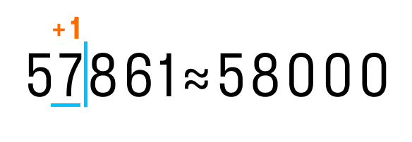
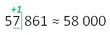
Давайте рассмотрим, как округлить число 57 861 до тысяч. Выполним первые два пункта из правил округления.
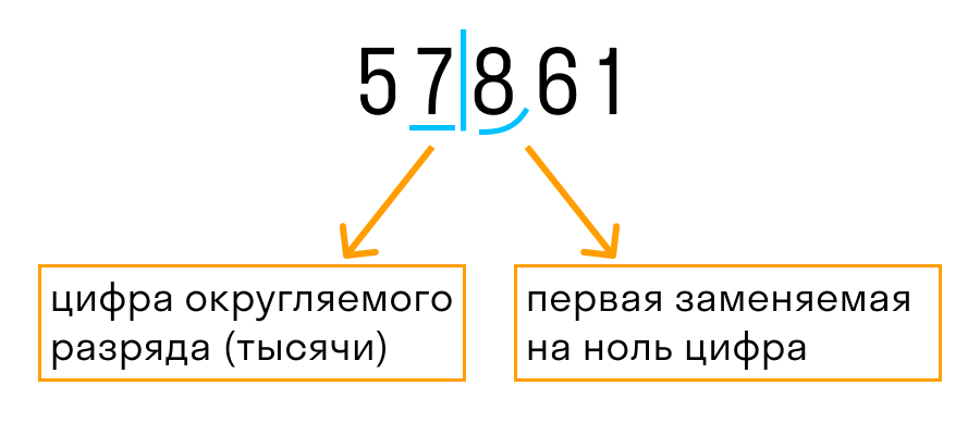
После подчеркнутой цифры стоит 8, значит к цифре разряда тысяч (в данном случае 7) прибавим 1. На месте цифр, отделенных вертикальной чертой, ставим нули.

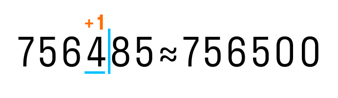
Теперь округлим 756 485 до сотен:
Округлим число 123 до десятков: 123 ≈ 120.
Округлим число 3581 до сотен: 3581 ≈ 3580.
Если в разряде, до которого производится округление, стоит цифра 9 и необходимо ее увеличить на единицу — в этом разряде записывается цифра 0, а цифра слева в соседнем старшем разряде увеличивается на 1.
Примеры:
- как округлить число 697 до десятков — 697 ≈ 700;
- как округлить число 980 до сотен — 980 ≈ 1000.
Иногда уместно записать округленный результат с сокращениями «тыс.» (тысяча), «млн.» (миллион) и «млрд.» (миллиард). Вот так:
- 7 882 000 = 7 882 тыс.
- 1 000 000 = 1 млн.
Округление десятичных дробей
Дробь — одна из форм записи частного чисел a и b, представленная в виде a/b. Есть два формата записи:
- обыкновенный вид — 1/2 или a/b,
- десятичный вид — 0,5.
В десятичной дроби знаменатель всегда равен 10, 100, 1000, 10 000 и т. д. Выходит, что десятичная дробь — это то, что получается, если разделить числитель на знаменатель. Такую дробь записывают в строчку через запятую, чтобы отделить целую часть от дробной. Вот так:
- 0,7
- 6,35
- 9,891
При округлении десятичных дробей следует быть особенно внимательным, потому что десятичная дробь состоит из целой и дробной части. И у каждой из этих частей есть свои разряды:
Разряды целой части:
- разряд единиц;
- разряд десятков;
- разряд сотен;
- разряд тысяч.
Разряды дробной части:
- разряд десятых;
- разряд сотых;
- разряд тысячных.
Разряд — это позиция, место расположения цифры в записи натурального числа. У каждого разряда есть свое название. Слева всегда располагаются старшие разряды, а справа — младшие.
Рассмотрим десятичную дробь 7396,1248. Здесь целая часть — 7396, а дробная — 1248. При этом у каждой из них есть свои разряды, которые важно не перепутать:

Чтобы округлить десятичную дробь, нужно в записи числа выбрать разряд, до которого производится округление.
То число, к которому дробь ближе, называют округленным значением числа.
Цифра, которая записана в данном разряде:
- не меняется, если следующая за ней справа цифра — 0,1, 2, 3 или 4;
- увеличивается на единицу, если за ней справа следует цифра — 5, 6, 7, 8 или 9.
Как округлить до десятых. Оставить одну цифру после запятой, остальные отбросить. Согласно правилу выше, если первая отбрасываемая цифра — 0, 1, 2, 3 или 4, то цифра после запятой остается той же. Если мы отбрасываем цифру 5, 6, 7, 8 или 9 — цифра после запятой увеличивается на единицу.
Как округлить до сотых. Оставить две цифры после запятой, остальные отбросить. И снова не забываем про правило: если следующая цифра 0, 1, 2, 4 — цифра в разряде сотых остается неизменной. Если же это 5, 6, 7, 8 или 9, то цифра в разряде сотых увеличится на 1.
Как округлить до целых. Заменить десятичную дробь ближайшим к ней целым числом. Ближайшим будет наименьшее расстояние. При этом если расстояние до приближенного значения числа с недостатком и расстояние до приближенного значения числа с избытком равны, то округляют в большую сторону.
Все цифры, которые стоят справа от данного разряда, заменяются нулями. Если эти нули стоят в дробной части числа, то их можно не писать.
Пример 1
256,43 ≈ 256,4 — округление до десятых;
4,578 ≈ 4,58 — округление до сотых;
17,935 ≈ 18 — округление до целых.
Если в разряде, до которого производится округление, стоит цифра 9 и необходимо ее увеличить на единицу, то в этом разряде записывается цифра 0, а цифра слева в предыдущем разряде увеличивается на 1.
Пример 2
79,7 ≈ 80 — округление до десятков;
0,099 ≈ 0,10 — округление до сотых.
Математическое округление и его правила быстро запомнится, если не лениться решать примеры и задачки из учебников 5 класса.
-
ОКРУГЛЕ́НИЕ, -я, ср. Действие по знач. глаг. округлить—округлять и состояние по знач. глаг. округлиться—округляться. [Литвинов] это сделал в видах увеличения и округления капитала. Тургенев, Дым.
Источник (печатная версия): Словарь русского языка: В 4-х
т. / РАН,
Ин-т лингвистич.
исследований; Под ред. А. П. Евгеньевой. — 4-е изд., стер. — М.: Рус. яз.;
Полиграфресурсы,
1999;
(электронная версия): Фундаментальная
электронная
библиотека
-
ОКРУГЛЕ’НИЕ, я, мн. нет, ср. (книжн.). Действие по глаг. округлить-округлять.
Источник: «Толковый словарь русского языка» под редакцией Д. Н. Ушакова (1935-1940);
(электронная версия): Фундаментальная
электронная
библиотека
-
округле́ние
1. действие по значению гл. округлять, округлить, округлеть, округлиться, округляться; придание чему-либо круглой формы ◆ Человек он был молодой, крупитчатый, с пунцовыми губами, пухлыми руками, с глазами выпяченными как у рака и с некоторой наклонностью к округлению брюшной полости. М. Е. Салтыков-Щедрин, «Современная идиллия», 1877–1883 г ◆ Гримёр, взглянув на эскиз, сказал, что для округления Серёжиного лица необходимо чуть нарастить щёки. Николай Шлиппенбах, «И явил нам Довлатов Петра», 2003 г. (цитата из НКРЯ) ◆ Произвольное округление углов и выступов здания ограничивает свободу в расстановке мебели. «„Элитное жильё“ — приближение к идеалу» // «Мир & Дом. City», 15 марта 2004 г. (цитата из НКРЯ)
2. результат такого действия; нечто округлое; округлость ◆ На юге горизонт замыкался слабо выраженными в дымке горами, высотами или просто слабыми округлениями песков. П. К. Козлов, «Географический дневник Тибетской экспедиции 1923–1926 гг.», 1925–1926 г (цитата из НКРЯ)
3. перен. придание окончательной, завершённой формы чего-либо; завершение, закругление ◆ — Он тут часа два слонялся… Я видел… — Мужик? — повторил кучер весьма равнодушным тоном, опять поглядел по сторонам, опять почесался и, должно быть для округления фразы, прибавил: — Нет, надо дубину хорошую, к примеру… По морде, чтобы в случае… да! Г. И. Успенский, «Наблюдения одного лентяя», (Очерки провинциальной жизни) / Из цикла «Разоренье», 1871 г. (цитата из НКРЯ)
4. перен. разг. достижение значительных размеров; увеличение ◆ Прежние владимирские князья постоянно стремились отрезать этот город от Рязанской области; московские имели ещё более причин желать Коломну: она запирала устье Москвы и была необходима для округления их волости. Д. И. Иловайский, «История Рязанского княжества», 1858 г. (цитата из НКРЯ) ◆ Он это сделал в видах увеличения и округления капитала; и он действительно если не увеличил, то округлил этот капитал, спустив излишние двадцать восемь гульденов. И. С. Тургенев, «Дым», 1867 г.
5. матем. действие по значению гл. округлять, округлить; выражение числа в круглых цифрах, с отбрасыванием дробных единиц счёта ◆ Разумеется, половину расходов я принимаю на себя, а для округления цифры, дай мне 50 рублей, и, таким образом, за мной будет 200. А. Ф. Кошко, «Очерки уголовного мира царской России», 1928 г. (цитата из НКРЯ) ◆ Конечно, такие расчёты подразумевают округление данных, а полученные результаты лежат в некотором интервале достоверности. Елена Кудрявцева, «Часовые службы погоды» // «Наука и жизнь», 2009 г. (цитата из НКРЯ)
6. результат такого действия; округлённое число
Источник: Викисловарь
Делаем Карту слов лучше вместе

Привет! Меня зовут Лампобот, я компьютерная программа, которая помогает делать
Карту слов. Я отлично
умею считать, но пока плохо понимаю, как устроен ваш мир. Помоги мне разобраться!
Спасибо! Я обязательно научусь отличать широко распространённые слова от узкоспециальных.
Насколько понятно значение слова глинобитный (прилагательное):
В приближенных вычислениях часто приходится округлять числа как приближенные, так и точные, т. е. отбрасывать одну или несколько последних цифр. Чтобы обеспечить наибольшую близость округленного числа к округляемому, соблюдаются следующие правила.
Правило 1. Если первая из отбрасываемых цифр больше чем 5, то последняя из сохраняемых
цифр усиливается, т. е. увеличивается на единицу. Усиление совершается и тогда, когда первая из отбрасываемых цифр равна 5, а за ней есть одна или несколько значащих цифр. (О случае, когда за отбрасываемой пятеркой нет цифр, см. ниже, правило 3.)
Пример 1. Округляя число 27,874 до трех значащих цифр, пишем 27,9. Третья цифра 8 усилена
до 9, так как первая отбрасываемая цифра 7 больше чем 5. Число 27,9 ближе к данному, чем неусиленное округленное число 27,8.
Пример 2. Округляя число 36,251 до первого десятичного знака, пишем 36,3. Цифра десятых 2 уси-
лена до 3, так как первая отбрасываемая цифра равна 5, а за ней есть значащая цифра 1. Число 36,3 ближе к данному (хотя и незначительно), чем неусиленное число 36,2.
Правило 2. Если первая из отбрасываемых цифр меньше чем 5, то усиления не делается.
Пример 3. Округляя число 27,48 до единиц, пишем 27. Это число ближе к данному, чем 28.
Правило 3. Если отбрасывается цифра 5, а за ней нет значащих цифр, то округление производится
на ближайшее четное число, т. е. последняя сохраняемая цифра оставляется неизменной, если она четная, и усиливается, если она нечетная. Почему применяется это правило, сказано ниже (см. замечание).
Пример 4. Округляя число 0,0465 до третьего десятичного знака, пишем 0,046. Усиления не делаем, так как последняя сохраняемая цифра 6 — четная. Число 0,046 столь же близко к данному, как 0,047.
Пример 5. Округляя число 0,935 до второго десятичного знака, пишем 0,94. Последняя сохраняемая цифра 3 усиливается, так как она нечетная.
Пример 6. Округляя числа 6,527; 0,456; 2,195; 1,450; 0,950; 4,851; 0,850; 0,05
до первого десятичного знака, получаем:
6,5; 0,5; 2,2; 1,4; 1,0; 4,9; 0,8; 0,0.
Замечание. Применяя правило 3 к округлению одного числа, мы не увеличиваем точность округления .Но при многочисленных округлениях избыточные числа будут встречаться
примерно столь же часто, как недостаточные. Взаимная компенсация погрешностей обеспечит наибольшую точность результата.
Правило 3 можно изменить и применять всегда округление на ближайшее нечетное число. Точность будет та же, но четные цифры удобнее, чем нечетные.
Существуют несколько методов округления числа:
ОКРУГЛЕНИЕ К БЛИЖАЙШЕМУ ЦЕЛОМУ
Округление к ближайшему целому до N-го знака осуществляется по следующему правилу:
- если N+1 знак
- если N+1 знак > 5, то N-ый знак увеличивают на единицу, а все знаки после N-го отбрасываются (обнуляются).
Примеры округления до 2 знаков после запятой:
2.4545 → 2.45
2.4564 → 2.46
По способам округления числа в случае когда N+1 знак равен 5, выделяются следующие виды округления к ближайшему целому:
- Математическое округление;
- Банковское округление;
- Случайное округление;
- Чередующееся округление.
Математическое округление в случае если N+1 знак = 5 увеличивает N-й знак на единицу, а все знаки после N-го отбрасываются (обнуляются).
Пример математического округления до 2-х знаков после запятой:
Данное округление в ABL реализовано в функции ROUND.
- iRnd – округляемое значение;
- n – знак до которого осуществляется округление.
Банковское округление отличается от математического тем, что предполагает округление в таком случае к ближайшему четному числу. Т.е. результатом округления числа 2.5 при математическом округлении будет 3, а при банковском 2.
Случайное округление осуществляет равновероятное округление числа 5 как в меньшую (N-ый знак остается без изменений) так и в большую (N-ый знак увеличивают на единицу) стороны. Например, в момент округления значения можно генерировать случайное целое число в пределах [0,1]. Если полученное число равно нулю, то округление осуществляется в меньшую сторону, если единице, то в большую.
Чередующееся округление осуществляет округление числа 5 поочередно то в меньшую, то в большую стороны. Данное округление очевидно применимо при необходимости округления массива чисел, а не единичного числа.
Округление мы часто используем в повседневной жизни. Если расстояние от дома до школы будет 503 метра. Мы можем сказать, округлив значение, что расстояние от дома до школы 500 метров. То есть мы приблизили число 503 к более легко воспринимающемуся числу 500. Например, булка хлеба весит 498 грамм, то можно сказать округлив результат, что булка хлеба весит 500 грамм.
Округление – это приближение числа к более “легкому” числу для восприятия человека.
В итоге округления получается приближенное число. Округление обозначается символом ≈, такой символ читается “приближённо равно”.
Можно записать 503≈500 или 498≈500.
Читается такая запись, как “пятьсот три приближенно равно пятистам” или “четыреста девяносто восемь приближенно равно пятистам”.
Разберем еще пример:
4 4 71≈4000 4 5 71≈5000
4 3 71≈4000 4 6 71≈5000
4 2 71≈4000 4 7 71≈5000
4 1 71≈4000 4 8 71≈5000
4 0 71≈4000 4 9 71≈5000
В данном примере было произведено округление чисел до разряда тысяч. Если посмотреть закономерность округления, то увидим, что в одном случае числа округляются в меньшую сторону, а в другом – в большую. После округления все остальные числа после разряда тысяч заменили на нули.
Правила округления чисел:
1) Если округляемая цифра равна 0, 1, 2, 3, 4, то цифра разряда до которого идет округление не меняется, а остальные числа заменяются нулями.
2) Если округляемая цифра равна 5, 6, 7, 8, 9, то цифра разряда до которого идет округление становиться на 1 больше, а остальные числа заменяются нулями.
1) Выполните округление до разряда десятков числа 364.
Разряд десятков в данном примере это число 6. После шестерки стоит число 4. По правилу округления цифра 4 разряд десятков не меняет. Записываем вместо 4 нуль. Получаем:
2) Выполните округление до разряда сотен числа 4 781.
Разряд сотен в данном примере это число 7. После семерки стоит цифра 8, которая влияет на то измениться ли разряд сотен или нет. По правилу округления цифра 8 увеличивает разряд сотен на 1, а остальные цифры заменяем нулями. Получаем:
3) Выполните округление до разряда тысяч числа 215 936.
Разряд тысяч в данном примере это число 5. После пятерки стоит цифра 9, которая влияет на то измениться ли разряд тысяч или нет. По правилу округления цифра 9 увеличивает разряд тысяч на 1, а остальные цифры заменяются нулями. Получаем:
21 5 9 36≈21 6 000
4) Выполните округление до разряда десятков тысяч числа 1 302 894.
Разряд тысяч в данном примере это число 0. После нуля стоит цифра 2, которая влияет на то измениться ли разряд десятков тысяч или нет. По правилу округления цифра 2 разряд десятков тысяч не меняет, заменяем на нуль этот разряд и все разряды младшие разряды. Получаем:
13 0 2 894≈13 0 0000
Если точное значение числа неважно, то значение числа округляют и можно выполнять вычислительные операции с приближенными значениями. Результат вычисления называют прикидкой результата действий.
Например: 598⋅23≈600⋅20≈12000 сравним с 598⋅23=13754
Прикидкой результата действий пользуются для того, чтобы быстро посчитать ответ.
Примеры на задания по теме округление:
Пример №1:
Определите до какого разряда сделано округление:
а) 3457987≈3500000 б)4573426≈4573000 в)16784≈17000
Вспомним какие бывают разряды на числе 3457987.
7 – разряд единиц,
8 – разряд десятков,
9 – разряд сотен,
7 – разряд тысяч,
5 – разряд десятков тысяч,
4 – разряд сотен тысяч,
3 – разряд миллионов.
Ответ: а) 3 4 57 987≈3 5 00 000 разряд сотен тысяч б) 4 57 3 426≈4 57 3 000 разряд тысяч в)1 6 7 841≈1 7 0 000 разряд десятков тысяч.
Пример №2:
Округлите число до разрядов 5 999 994: а) десятков б) сотен в) миллионов.
Ответ: а) 5 999 99 4 ≈5 999 990 б) 5 999 9 9 4≈6 000 000 (т.к. разряды сотен, тысяч, десятков тысяч, сотен тысяч цифра 9, каждый разряд увеличился на 1) 5 9 99 994≈6 000 000.
В разных сферах могут применяться различные методы округления. Во всех этих методах «лишние» знаки обнуляют (отбрасывают), а предшествующий им знак корректируется по какому-либо правилу.
- Округление к ближайшему целому (англ.rounding ) — наиболее часто используемое округление, при котором число округляется до целого, модуль разности с которым у этого числа минимален. В общем случае, когда число в десятичной системе округляют до N-ого знака, правило может быть сформулировано следующим образом:
- если N+1 знак Например: 11,9 → 12; −0,9 → −1; −1,1 → −1; 2,5 → 3.
- Округление к меньшему по модулю (округление к нулю, целое англ.fix, truncate, integer ) — самое «простое» округление, поскольку после обнуления «лишних» знаков предшествующий знак сохраняют. Например, 11,9 → 11; −0,9 → 0; −1,1 → −1).
- Округление к большему (округление к +∞, округление вверх, англ.ceiling ) — если обнуляемые знаки не равны нулю, предшествующий знак увеличивают на единицу, если число положительное, или сохраняют, если число отрицательное. В экономическом жаргоне — округление в пользу продавца, кредитора (лица, получающего деньги). В частности, 2,6 → 3, −2,6 → −2.
- Округление к меньшему (округление к −∞, округление вниз, англ.floor ) — если обнуляемые знаки не равны нулю, предшествующий знак сохраняют, если число положительное, или увеличивают на единицу, если число отрицательное. В экономическом жаргоне — округление в пользу покупателя, дебитора (лица, отдающего деньги). Здесь 2,6 → 2, −2,6 → −3.
- Округление к большему по модулю (округление к бесконечности, округление от нуля) — относительно редко используемая форма округления. Если обнуляемые знаки не равны нулю, предшествующий знак увеличивают на единицу.
Варианты округления 0,5 к ближайшему целому
Отдельного описания требуют правила округления для специального случая, когда (N+1)-й знак = 5, а последующие знаки равны нулю. Если во всех остальных случаях округление до ближайшего целого обеспечивает меньшую погрешность округления, то данный частный случай характерен тем, что для однократного округления формально безразлично, производить его «вверх» или «вниз» — в обоих случаях вносится погрешность ровно в 1/2 младшего разряда. Существуют следующие варианты правила округления до ближайшего целого для данного случая:
- Математическое округление — округление всегда в бо́льшую по модулю сторону (предыдущий разряд всегда увеличивается на единицу).
- Банковское округление (англ.banker’s rounding ) — округление для этого случая происходит к ближайшему чётному, то есть 2,5 → 2, 3,5 → 4.
- Случайное округление — округление происходит в меньшую или большую сторону в случайном порядке, но с равной вероятностью (может использоваться в статистике).
- Чередующееся округление — округление происходит в меньшую или большую сторону поочерёдно.
Во всех вариантах в случае, когда (N+1)-й знак не равен 5 или последующие знаки не равны нулю, округление происходит по обычным правилам: 2,49 → 2; 2,51 → 3.
Математическое округление просто формально соответствует общему правилу округления (см. выше). Его недостатком является то, что при округлении большого числа значений может происходить накопление ошибки округления. Типичный пример: округление до целых рублей денежных сумм. Так, если в реестре из 10000 строк окажется 100 строк с суммами, содержащими в части копеек значение 50 (а это вполне реальная оценка), то при округлении всех таких строк «вверх» сумма «итого» по округлённому реестру окажется на 50 рублей больше точной.
Три остальных варианта как раз и придуманы для того, чтобы уменьшить общую погрешность суммы при округлении большого количества значений. Округление «до ближайшего чётного» исходит из предположения, что при большом числе округляемых значений, имеющих 0,5 в округляемом остатке, в среднем половина окажется слева, а половина — справа от ближайшего чётного, таким образом, ошибки округления взаимно погасятся. Строго говоря, предположение это верно лишь тогда, когда набор округляемых чисел обладает свойствами случайного ряда, что обычно верно в бухгалтерских приложениях, где речь идёт о ценах, суммах на счетах и так далее. Если же предположение будет нарушено, то и округление «до чётного» может приводить к систематическим ошибкам. Для таких случаев лучше работают два следующих метода.
Два последних варианта округления гарантируют, что примерно половина специальных значений будет округлена в одну сторону, половина — в другую. Но реализация таких методов на практике требует дополнительных усилий по организации вычислительного процесса.
Применения
Округление используется для того, чтобы работать с числами в пределах того количества знаков, которое соответствует реальной точности параметров вычислений (если эти значения представляют собой измеренные тем или иным образом реальные величины), реально достижимой точности вычислений либо желаемой точности результата. В прошлом округление промежуточных значений и результата имело прикладное значение (так как при расчётах на бумаге или с помощью примитивных устройств типа абака учёт лишних десятичных знаков может серьёзно увеличить объём работы). Сейчас оно остаётся элементом научной и инженерной культуры. В бухгалтерских приложениях, кроме того, использование округлений, в том числе промежуточных, может требоваться для защиты от вычислительных ошибок, связанных с конечной разрядностью вычислительных устройств.
Использование округлений при работе с числами ограниченной точности
Реальные физические величины всегда измеряются с некоторой конечной точностью, которая зависит от приборов и методов измерения и оценивается максимальным относительным или абсолютным отклонением неизвестного действительного значения от измеренного, что в десятичном представлении значения соответствует либо определённому числу значащих цифр, либо определённой позиции в записи числа, все цифры после (правее) которой являются незначащими (лежат в пределах ошибки измерения). Сами измеренные параметры записываются с таким числом знаков, чтобы все цифры были надёжными, возможно, последняя — сомнительной. Погрешность при математических операциях с числами ограниченной точности сохраняется и изменяется по известным математическим законам, поэтому когда в дальнейших вычислениях возникают промежуточные значения и результаты с больши́м числом цифр, из этих цифр только часть являются значимыми. Остальные цифры, присутствуя в значениях, фактически не отражают никакой физической реальности и лишь отнимают время на вычисления. Вследствие этого промежуточные значения и результаты при вычислениях с ограниченной точностью округляют до того количества знаков, которое отражает реальную точность полученных значений. На практике обычно рекомендуется при длинных «цепочных» ручных вычислениях сохранять в промежуточных значениях на одну цифру больше. При использовании компьютера промежуточные округления в научно-технических приложениях чаще всего теряют смысл, и округляется только результат.
Так, например, если задана сила 5815 гс с точностью до грамма силы и длина плеча 1,4 м с точностью до сантиметра, то момент силы в кгс по формуле  , в случае формального расчёта со всеми знаками, окажется равным: 5,815 кгс • 1,4 м = 8,141 кгс•м. Однако если учесть погрешность измерения, то мы получим, что предельная относительная погрешность первого значения составляет 1/5815 ≈ 1,7•10 −4 , второго — 1/140 ≈ 7,1•10 −3 , относительная погрешность результата по правилу погрешности операции умножения (при умножении приближённых величин относительные погрешности складываются) составит 7,3•10 −3 , что соответствует максимальной абсолютной погрешности результата ±0,059 кгс•м! То есть в реальности, с учётом погрешности, результат может составлять от 8,082 до 8,200 кгс•м, таким образом, в рассчитанном значении 8,141 кгс•м полностью надёжной является только первая цифра, даже вторая — уже сомнительна! Корректным будет округление результата вычислений до первой сомнительной цифры, то есть до десятых: 8,1 кгс•м, или, при необходимости более точного указания рамок погрешности, представить его в виде, округлённом до одного-двух знаков после запятой с указанием погрешности: 8,14 ± 0,06 кгс•м.
Эмпирические правила арифметики с округлениями
В тех случаях, когда нет необходимости в точном учёте вычислительных погрешностей, а требуется лишь приблизительно оценить количество точных цифр в результате расчёта по формуле, можно пользоваться набором простых правил округлённых вычислений [1] :
- Все исходные значения округляются до реальной точности измерений и записываются с соответствующим числом значащих цифр, так, чтобы в десятичной записи все цифры были надёжными (допускается, чтобы последняя цифра была сомнительной). При необходимости значения записываются со значащими правыми нулями, чтобы в записи указывалось реальное число надёжных знаков (например, если длина в 1 м реально измерена с точностью до сантиметров, записывается «1,00 м», чтобы было видно, что в записи надёжны два знака после запятой), или точность явно указывается (например, 2500±5 м — здесь надёжными являются только десятки, до них и следует округлять).
- Промежуточные значения округляются с одной «запасной» цифрой.
- При сложении и вычитании результат округляется до последнего десятичного знака наименее точного из параметров (например, при вычислении значения 1,00 м + 1,5 м + 0,075 м результат округляется до десятых метра, то есть до 2,6 м). При этом рекомендуется выполнять вычисления в таком порядке, чтобы избегать вычитания близких по величине чисел и производить действия над числами по возможности в порядке возрастания их модулей.
- При умножении и делении результат округляется до наименьшего числа значащих цифр, которое имеют параметры (например, при вычислении скорости равномерного движения тела на дистанции 2,5•10 2 м, за 600 с результат должен быть округлён до 4,2 м/с, поскольку именно две цифры имеет расстояние, а время — три, предполагая, что все цифры в записи — значащие).
- При вычислении значения функции f(x) требуется оценить значение модуля производной этой функции в окрестности точки вычисления. Если (|f'(x)| ≤ 1), то результат функции точен до того же десятичного разряда, что и аргумент. В противном случае результат содержит меньше точных десятичных разрядов на величину log10(|f'(x)|), округлённую до целого в большую сторону.
Несмотря на нестрогость, приведённые правила достаточно хорошо работают на практике, в частности, из-за достаточно высокой вероятности взаимопогашения ошибок, которая при точном учёте погрешностей обычно не учитывается.
Ошибки
Довольно часто встречаются злоупотребления некруглыми числами. Например:
- Записывают числа, имеющие невысокую точность, в неокруглённом виде. В статистике: если 4 человека из 17 ответили «да», то пишут «23,5 %» (в то время как верно «24 %»).
- Пользователи стрелочных приборов иногда размышляют так: «стрелка остановилась между 5,5 и 6 ближе к 6, пусть будет 5,8» — это также запрещено (градуировка прибора как правило соответствует его реальной точности). В таком случае надо говорить «5,5» или «6».
Приближенные значения
В обычной жизни мы часто встречаем два вида чисел: точные и приближенные. И если точные до сих пор были понятны, то с приближенными предстоит познакомиться в 5 классе.
У квадрата четыре стороны — число 4 невозможно оспорить, оно точное. У каждого окна есть своя ширина, и его параметры однозначно точные. А вот арбуз весит примерно 5 кг, и никакие весы не покажут абсолютно точный вес. И градусник показывает температуру с небольшой погрешностью. Поэтому вместо точных значений величин иногда можно использовать приближенные значения.
Онлайн-школа Skysmart приглашает детей и подростков на курсы по математике — за интересными задачами, новыми прикладными знаниями и хорошими оценками!
Примерчики
-
Весы показывают, что арбуз весит 5,160 кг. Можно сказать, что арбуз весит примерно 5 кг. Это приближенное значение с недостатком.
-
Часы показывают время: два часа дня и пятьдесят пять минут. В разговоре про время можно сказать: «почти три» или «время около трех». Это значение времени с избытком.
-
Если длина платья 1 м 30 см, то 1 м — это приближенное значение длины с недостатком, а 1,5 м — это приближенное значение длины с избытком.
Приближенное значение — число, которое получилось после округления.
Для записи результата округления используют знак «приблизительно равно» — ≈.
Округлить можно любое число — для всех чисел работают одни и те же правила.
Округлить число значит сократить его значение до нужного разряда, например, до сотых, десятков или тысячных, остальные значения откидываются. Это нужно в случаях, когда полная точность не нужна или невозможна.
Получай лайфхаки, статьи, видео и чек-листы по обучению на почту
Реши домашку по математике на 5.
Подробные решения помогут разобраться в самой сложной теме.
Округление натуральных чисел
Натуральные числа — это числа, которые мы используем, чтобы посчитать что-то конкретное, осязаемое. Вот они: 1, 2, 3, 4, 5, 6, 7, 8, 9, 10, 11, 12, 13 и так далее.
Особенности натуральных чисел:
- Наименьшее натуральное число: единица (1).
- Наибольшего натурального числа не существует. Натуральный ряд бесконечен.
- У натурального ряда каждое следующее число больше предыдущего на единицу: 1, 2, 3, 4, 5, 6, 7.
Округление натурального числа — это замена его таким ближайшим по значению числом, у которого одна или несколько последних цифр в его записи заменены нулями.
Чтобы округлить натуральное число, нужно в записи числа выбрать разряд, до которого производится округление.
Правила округления чисел:
- Подчеркнуть цифру разряда, до которого надо округлить число.
- Отделить все цифры справа от этого разряда вертикальной чертой.
- Если справа от подчеркнутой цифры стоит 0,1, 2, 3 или 4 — все цифры, которые отделены справа, заменяем нулями. Цифру разряда, до которой округляли, оставляем без изменений.
- Если справа от подчеркнутой цифры стоит 5, 6, 7, 8 или 9 — все цифры, которые отделены справа, заменяем нулями. К цифре разряда, до которой округляли, прибавляем 1.
Давайте рассмотрим, как округлить число 57 861 до тысяч. Выполним первые два пункта из правил округления.

После подчеркнутой цифры стоит 8, значит к цифре разряда тысяч (в данном случае 7) прибавим 1. На месте цифр, отделенных вертикальной чертой, ставим нули.
Теперь округлим 756 485 до сотен:

Округлим число 123 до десятков: 123 ≈ 120.
Округлим число 3581 до сотен: 3581 ≈ 3580.
Если в разряде, до которого производится округление, стоит цифра 9 и необходимо ее увеличить на единицу — в этом разряде записывается цифра 0, а цифра слева в соседнем старшем разряде увеличивается на 1.
Примеры:
- как округлить число 697 до десятков — 697 ≈ 700;
- как округлить число 980 до сотен — 980 ≈ 1000.
Иногда уместно записать округленный результат с сокращениями «тыс.» (тысяча), «млн.» (миллион) и «млрд.» (миллиард). Вот так:
- 7 882 000 = 7 882 тыс.
- 1 000 000 = 1 млн.
Округление десятичных дробей
Дробь — одна из форм записи частного чисел a и b, представленная в виде a/b. Есть два формата записи:
- обыкновенный вид — 1/2 или a/b,
- десятичный вид — 0,5.
В десятичной дроби знаменатель всегда равен 10, 100, 1000, 10 000 и т. д. Выходит, что десятичная дробь — это то, что получается, если разделить числитель на знаменатель. Такую дробь записывают в строчку через запятую, чтобы отделить целую часть от дробной. Вот так:
- 0,7
- 6,35
- 9,891
При округлении десятичных дробей следует быть особенно внимательным, потому что десятичная дробь состоит из целой и дробной части. И у каждой из этих частей есть свои разряды:
Разряды целой части:
- разряд единиц;
- разряд десятков;
- разряд сотен;
- разряд тысяч.
Разряды дробной части:
- разряд десятых;
- разряд сотых;
- разряд тысячных.
Разряд — это позиция, место расположения цифры в записи натурального числа. У каждого разряда есть свое название. Слева всегда располагаются старшие разряды, а справа — младшие.
Рассмотрим десятичную дробь 7396,1248. Здесь целая часть — 7396, а дробная — 1248. При этом у каждой из них есть свои разряды, которые важно не перепутать:

Чтобы округлить десятичную дробь, нужно в записи числа выбрать разряд, до которого производится округление.
То число, к которому дробь ближе, называют округленным значением числа.
Цифра, которая записана в данном разряде:
- не меняется, если следующая за ней справа цифра — 0,1, 2, 3 или 4;
- увеличивается на единицу, если за ней справа следует цифра — 5, 6, 7, 8 или 9.
Как округлить до десятых. Оставить одну цифру после запятой, остальные отбросить. Согласно правилу выше, если первая отбрасываемая цифра — 0, 1, 2, 3 или 4, то цифра после запятой остается той же. Если мы отбрасываем цифру 5, 6, 7, 8 или 9 — цифра после запятой увеличивается на единицу.
Как округлить до сотых. Оставить две цифры после запятой, остальные отбросить. И снова не забываем про правило: если следующая цифра 0, 1, 2, 4 — цифра в разряде сотых остается неизменной. Если же это 5, 6, 7, 8 или 9, то цифра в разряде сотых увеличится на 1.
Как округлить до целых. Заменить десятичную дробь ближайшим к ней целым числом. Ближайшим будет наименьшее расстояние. При этом если расстояние до приближенного значения числа с недостатком и расстояние до приближенного значения числа с избытком равны, то округляют в большую сторону.
Все цифры, которые стоят справа от данного разряда, заменяются нулями. Если эти нули стоят в дробной части числа, то их можно не писать.
Пример 1
256,43 ≈ 256,4 — округление до десятых;
4,578 ≈ 4,58 — округление до сотых;
17,935 ≈ 18 — округление до целых.
Если в разряде, до которого производится округление, стоит цифра 9 и необходимо ее увеличить на единицу, то в этом разряде записывается цифра 0, а цифра слева в предыдущем разряде увеличивается на 1.
Пример 2
79,7 ≈ 80 — округление до десятков;
0,099 ≈ 0,10 — округление до сотых.
Математическое округление и его правила быстро запомнится, если не лениться решать примеры и задачки из учебников 5 класса.
В данной публикации мы рассмотрим, что из себя представляет округление числа, по каким правилам выполняется, а также разберем практический пример по этой теме.
-
Что такое округление числа
- Правила округления
- Практический пример
Что такое округление числа
Во время выполнения тех или иных расчетов довольно часто требуется округлить полученный результат или использовать округленные значения в вычислениях.
Округление – это замена числа на приближенное ему значение, скажем так, “сокращенное” до определенной цифры или знака.
Натуральные числа можно округлить до любых разрядов (десятков, сотен, тысяч и т.д.) – всё зависит от исходного значения и требуемой точности.
Получаемое в результате округления число называется округленным или приближенным.
Для округления предусмотрен специальный символ – “≈“, после которого пишется округленное число. Произносится как “приближенно равно”.
Правила округления
- Отмечаем цифру, расположенную в том разряде, до которого требуется выполнить округление.
- Отделяем все цифры, находящиеся справа от выбранного раздела.
- Далее возможны два варианта:
- если справа от отмеченного разряда стоят цифры 0, 1, 2, 3 или 4, то вместо всех отделенных справа цифр мы пишем ноль. Сама цифра разряда остается той же.
- если справа от выбранного разряда стоят цифры 5, 6, 7, 8 или 9, то все отделенные цифры, также, меняем на нули, а к самой цифре разряда прибавляем единицу.
Примечание: Округление десятичных дробей мы подробное рассмотрели в отдельной публикации.
Практический пример
Выполним округление числа 654 719 до тысяч.
Решение:
Руководствуясь правилами выше отметим нужный разряд и вертикальной черточкой отделим от него цифры справа.

После округляемого разряда стоит цифра 7, следовательно к разряду тысяч прибавляем единицу (4 + 1), а отмеченные красным цифры меняем на нули.
Таким образом, получаем: 654 719 ≈ 655 000.
Это же число, округленное до:
- сотен: ≈ 655 700
- десятков: ≈ 655 720
Примечание: округленные результаты обычно пишутся без нулей, при этом к ним обязательно добавляется сокращение, соответствующее точности округления: “сот”, “тыс”, “млн” и т.д. Например, 126 415 ≈ 126 тыс.
Как округлять числа
Вспоминаем полезное правило из школьной программы.

Что такое округление числа
Округление — это замена числа близким по значению, у которого на конце стоит ноль. Тогда исходное число и станет круглым. Например, круглыми являются числа 10, 20, 100, 730, 1 420, 15 000.
Результат округления называется приближённым значением данного числа и указывается после знака ≈ («приблизительно равно»).
Как округлять числа
Натуральные числа
Все числа, в которых больше одного знака, имеют разряды. Это место, на котором в числе стоит та или иная цифра. Например, в числе 342 три разряда: сотен (три сотни), десятков (четыре десятка) и единиц (две единицы). Соответственно, округлять числа можно до десятков, сотен, тысяч и так далее.
При округлении цифры в ненужных нам разрядах заменяются нулями (по сути, отбрасываются), а цифра в нужном разряде либо изменяется в большую сторону, либо остаётся неизменной. Это зависит от того, какая цифра стоит за ней. Если от 0 до 4, то ничего не происходит. Если от 5 до 9, тогда к разряду прибавляется единица.
Возьмём число 21 769. Его можно округлить следующим образом:
- До десятков. Находим количество десятков в числе 21 769 — их шесть. За шестёркой стоит цифра 9, значит, при округлении разряд десятков увеличится на один. То есть ответ — 21 770.
- До сотен. Находим количество сотен в числе 21 769 — их семь. Теперь проверяем цифру за семёркой — это 6, соответственно, к разряду сотен прибавляем единицу. Результат — 21 800.
- До тысяч. Находим количество тысяч — их 21. За единицей стоит семёрка, значит, при округлении числа разряд тысяч увеличиваем на один и получаем 22 000.
Дробные числа
При округлении дробей действуют точно такие же правила, как и при округлении натуральных чисел. Только нужно быть более внимательным, потому что разрядов в дробях больше — они есть и в целой части (единицы, десятки, сотни, тысячи и т. д.), и в дробной (десятые, сотые, тысячные и т. д.).
Например, возьмём десятичную дробь 45,836. Её можно округлить так:
- до сотых → 45,84;
- до десятых → 45,8;
- до целого → 46;
- до десятков → 50.
Когда пригодится округление чисел
Округление помогает в самых разных случаях. Например, когда нужно прикинуть результат умножения больших чисел. Допустим, вы хотите представить, сколько будет 738 × 46. По правилам округления, это приблизительно равно 700 × 50. Получается: 738 × 46 ≈ 700 × 50 ≈ 35 000. А точный результат умножения равен 33 948.
Правила округления чисел пригодятся не только при решении задачек, но и когда нужно примерно рассчитать стоимость чего‑то, чтобы понять, укладывается ли она в ваш бюджет или нет.
Также к округлению прибегают, когда абсолютная точность просто не важна. Например, если знакомые из другого города спросят вас, сколько людей живёт в вашем, вы вряд ли будете называть число до десятков и единиц, даже если знаете его. Вы, скорее, скажете, что в нём живёт «примерно четыреста тысяч» или «около миллиона» человек.
Читайте также 🧐
- Какого числа не хватает? 10 интересных заданий на поиск закономерностей
- Простой математический лайфхак, как быстро высчитать процент от числа
- Гимнастика для ума: 10 увлекательных задач с числами
Числа округляют, когда полная точность не нужна или невозможна.
Запомните!
![]()
Округлить число до определенной цифры (знака),
значит заменить его близким по значению числом с нулями на конце.
Натуральные числа округляют до десятков, сотен, тысяч и т.д. Названия
цифр в разрядах натурального числа можно вспомнить
в теме натуральные числа.
В зависимости от того, до какого разряда надо округлить число, мы заменяем нулями цифру в разрядах единиц,
десятков и т.д.
Если число округляется до десятков, то нулями заменяем цифру в разряде единицы.
Если число округляется до сотен, то цифра ноль должна стоять и в разряде единиц, и в разряде десятков.
Запомните!
![]()
Число, полученное при округлении, называют приближённым значением данного числа.
Записывают результат округления после специального знака «≈». Этот знак читается как «приближённо равно».
При округлении натурального числа до какого-либо разряда надо воспользоваться правилами округления.
- Подчеркнуть цифру разряда, до которого надо округлить число.
- Отделить все цифры, стоящие справа этого разряда вертикальной чертой.
- Если справа от подчёркнутой цифры стоит цифра 0, 1, 2, 3 или
4
, то все
цифры, которые отделены справа, заменяются нулями. Цифру разряда, до которой округляли, оставляем без изменений. - Если справа от подчёркнутой цифры стоит цифра 5, 6, 7, 8 или
9
, то все
цифры, которые отделены справа, заменяются нулями, а к цифре разряда, до которой
округляли, прибавляется 1.
Поясним на примере. Округлим 57 861 до тысяч. Выполним первые два пункта из правил округления.

После подчёркнутой цифры стоит цифра 8, значит к цифре разряда тысяч (у нас это
7) прибавим 1, а все
цифры, отделённые вертикальной чертой заменим нулями.
Теперь округлим 756 485 до сотен.

Округлим 364 до десятков.
36|4 ≈ 360 — в разряде единиц стоит
4, поэтому мы оставляем 6 в разряде десятков без изменений.
На числовой оси число 364 заключено между двумя «круглыми» числами
360 и 370. Эти два числа
называют приближёнными значениями числа 364 с точностью до десятков.
Число 360 — приближённое значение с недостатком,
а число 370 — приближённое значение с избытком.
В нашем случае, округлив 364 до десятков, мы получили, 360 — приближённое значение с недостатком.
Округлённые результаты часто записывают без нулей, добавляя
сокращения «тыс.» (тысяча), «млн.» (миллион) и «млрд.» (миллиард).
Примеры:
- 8 659 000 = 8 659 тыс.
- 3 000 000 = 3 млн.
Округление также применяется для прикидочной проверки ответа в вычислениях.
Пусть нам нужно посчитать:
794 · 52 =
До точного вычисления сделаем прикидку ответа, округлив множители до наивысшего разряда.
794 · 52 ≈ 800 · 50 ≈ 40 000
Делаем вывод, что ответ будет близок к 40 000.
794 · 52 = 41 228
Аналогично можно выполнять прикидку округлением и при делении чисел.
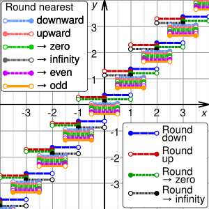
Graphs of the result, y, of rounding x using different methods. For clarity, the graphs are shown displaced from integer y values. In the SVG file, hover over a method to highlight it and, in SMIL-enabled browsers, click to select or deselect it.
Rounding means replacing a number with an approximate value that has a shorter, simpler, or more explicit representation. For example, replacing $23.4476 with $23.45, the fraction 312/937 with 1/3, or the expression √2 with 1.414.
Rounding is often done to obtain a value that is easier to report and communicate than the original. Rounding can also be important to avoid misleadingly precise reporting of a computed number, measurement, or estimate; for example, a quantity that was computed as 123,456 but is known to be accurate only to within a few hundred units is usually better stated as «about 123,500».
On the other hand, rounding of exact numbers will introduce some round-off error in the reported result. Rounding is almost unavoidable when reporting many computations – especially when dividing two numbers in integer or fixed-point arithmetic; when computing mathematical functions such as square roots, logarithms, and sines; or when using a floating-point representation with a fixed number of significant digits. In a sequence of calculations, these rounding errors generally accumulate, and in certain ill-conditioned cases they may make the result meaningless.
Accurate rounding of transcendental mathematical functions is difficult because the number of extra digits that need to be calculated to resolve whether to round up or down cannot be known in advance. This problem is known as «the table-maker’s dilemma».
Rounding has many similarities to the quantization that occurs when physical quantities must be encoded by numbers or digital signals.
A wavy equals sign (≈: approximately equal to) is sometimes used to indicate rounding of exact numbers, e.g., 9.98 ≈ 10. This sign was introduced by Alfred George Greenhill in 1892.[1]
Ideal characteristics of rounding methods include:
- Rounding should be done by a function. This way, when the same input is rounded in different instances, the output is unchanged.
- Calculations done with rounding should be close to those done without rounding.
- As a result of (1) and (2), the output from rounding should be close to its input, often as close as possible by some metric.
- To be considered rounding, the range will be a subset of the domain, in general discrete. A classical range is the integers, Z.
- Rounding should preserve symmetries that already exist between the domain and range. With finite precision (or a discrete domain), this translates to removing bias.
- A rounding method should have utility in computer science or human arithmetic where finite precision is used, and speed is a consideration.
Because it is not usually possible for a method to satisfy all ideal characteristics, many different rounding methods exist.
As a general rule, rounding is idempotent;[2] i.e., once a number has been rounded, rounding it again will not change its value. Rounding functions are also monotonic; i.e., rounding a larger number gives a larger or equal result than rounding a smaller number[clarification needed]. In the general case of a discrete range, they are piecewise constant functions.
Types of rounding[edit]
Typical rounding problems include:
| Rounding problem | Example input | Result | Rounding criterion |
|---|---|---|---|
| Approximating an irrational number by a fraction | π | 22 / 7 | 1-digit-denominator |
| Approximating a rational number by another fraction with smaller numerator and denominator | 399 / 941 | 3 / 7 | 1-digit-denominator |
| Approximating a fraction, which have periodic decimal expansion, by a finite decimal fraction | 5 / 3 | 1.6667 | 4 decimal places |
| Approximating a fractional decimal number by one with fewer digits | 2.1784 | 2.18 | 2 decimal places |
| Approximating a decimal integer by an integer with more trailing zeros | 23,217 | 23,200 | 3 significant figures |
| Approximating a large decimal integer using scientific notation | 300,999,999 | 3.01 × 10⁸ | 3 significant figures |
| Approximating a value by a multiple of a specified amount | 48.2 | 45 | Multiple of 15 |
| Rounding each one of a finite set of real numbers (mostly fractions) to an integer (sometimes the second-nearest integer) so that the sum of the rounded numbers equals the rounded sum of the numbers (needed e.g. [1] for the apportionment of seats, implemented e.g. by the largest remainder method, see Mathematics of apportionment, and [2] for distributing the total VAT of an invoice to its items) | {3/12, 4/12, 5/12} | {0, 0, 1} | Sum of rounded elements equals rounded sum of elements |
Rounding to integer[edit]
The most basic form of rounding is to replace an arbitrary number by an integer. All the following rounding modes are concrete implementations of an abstract single-argument «round()» procedure. These are true functions (with the exception of those that use randomness).
Directed rounding to an integer[edit]
These four methods are called directed rounding, as the displacements from the original number x to the rounded value y are all directed toward or away from the same limiting value (0, +∞, or −∞). Directed rounding is used in interval arithmetic and is often required in financial calculations.
If x is positive, round-down is the same as round-toward-zero, and round-up is the same as round-away-from-zero. If x is negative, round-down is the same as round-away-from-zero, and round-up is the same as round-toward-zero. In any case, if x is an integer, y is just x.
Where many calculations are done in sequence, the choice of rounding method can have a very significant effect on the result. A famous instance involved a new index set up by the Vancouver Stock Exchange in 1982. It was initially set at 1000.000 (three decimal places of accuracy), and after 22 months had fallen to about 520 — whereas stock prices had generally increased in the period. The problem was caused by the index being recalculated thousands of times daily, and always being rounded down to 3 decimal places, in such a way that the rounding errors accumulated. Recalculating with better rounding gave an index value of 1098.892 at the end of the same period.[3]
For the examples below, sgn(x) refers to the sign function applied to the original number, x.
Rounding down[edit]
- round down (or take the floor, or round toward negative infinity): y is the largest integer that does not exceed x.

For example, 23.7 gets rounded to 23, and −23.2 gets rounded to −24.
Rounding up[edit]
- round up (or take the ceiling, or round toward positive infinity): y is the smallest integer that is not less than x.

For example, 23.2 gets rounded to 24, and −23.7 gets rounded to −23.
Rounding toward zero[edit]
- round toward zero (or truncate, or round away from infinity): y is the integer that is closest to x such that it is between 0 and x (included); i.e. y is the integer part of x, without its fraction digits.

For example, 23.7 gets rounded to 23, and −23.7 gets rounded to −23.
Rounding away from zero[edit]
- round away from zero (or round toward infinity): y is the integer that is closest to 0 (or equivalently, to x) such that x is between 0 and y (included).

For example, 23.2 gets rounded to 24, and −23.2 gets rounded to −24.
Rounding to the nearest integer[edit]
Rounding a number x to the nearest integer requires some tie-breaking rule for those cases when x is exactly half-way between two integers — that is, when the fraction part of x is exactly 0.5.
If it were not for the 0.5 fractional parts, the round-off errors introduced by the round to nearest method would be symmetric: for every fraction that gets rounded down (such as 0.268), there is a complementary fraction (namely, 0.732) that gets rounded up by the same amount.
When rounding a large set of fixed-point numbers with uniformly distributed fractional parts, the rounding errors by all values, with the omission of those having 0.5 fractional part, would statistically compensate each other. This means that the expected (average) value of the rounded numbers is equal to the expected value of the original numbers when numbers with fractional part 0.5 from the set are removed.
In practice, floating-point numbers are typically used, which have even more computational nuances because they are not equally spaced.
Rounding half up[edit]
The following tie-breaking rule, called round half up (or round half toward positive infinity), is widely used in many disciplines.[citation needed] That is, half-way values of x are always rounded up.
- If the fractional part of x is exactly 0.5, then y = x + 0.5

For example, 23.5 gets rounded to 24, and −23.5 gets rounded to −23.
However, some programming languages (such as Java, Python) define their half up as round half away from zero here.[4][5]
This method only requires checking one digit to determine rounding direction in two’s complement and similar representations.
Rounding half down[edit]
One may also use round half down (or round half toward negative infinity) as opposed to the more common round half up.
- If the fractional part of x is exactly 0.5, then y = x − 0.5

For example, 23.5 gets rounded to 23, and −23.5 gets rounded to −24.
However, some programming languages (such as Java, Python) define their half down as round half toward zero here.[4][5]
Rounding half toward zero[edit]
One may also round half toward zero (or round half away from infinity) as opposed to the conventional round half away from zero.
- If the fractional part of x is exactly 0.5, then y = x − 0.5 if x is positive, and y = x + 0.5 if x is negative.

For example, 23.5 gets rounded to 23, and −23.5 gets rounded to −23.
This method treats positive and negative values symmetrically, and therefore is free of overall positive/negative bias if the original numbers are positive or negative with equal probability. It does, however, still have bias toward zero.
Rounding half away from zero[edit]
The other tie-breaking method commonly taught and used is the round half away from zero (or round half toward infinity), namely:
- If the fractional part of x is exactly 0.5, then y = x + 0.5 if x is positive, and y = x − 0.5 if x is negative.

For example, 23.5 gets rounded to 24, and −23.5 gets rounded to −24.
This can be more efficient on binary computers because only the first omitted bit needs to be considered to determine if it rounds up (on a 1) or down (on a 0). This is one method used when rounding to significant figures due to its simplicity.
This method, also known as commercial rounding,[citation needed] treats positive and negative values symmetrically, and therefore is free of overall positive/negative bias if the original numbers are positive or negative with equal probability. It does, however, still have bias away from zero.
It is often used for currency conversions and price roundings (when the amount is first converted into the smallest significant subdivision of the currency, such as cents of a euro) as it is easy to explain by just considering the first fractional digit, independently of supplementary precision digits or sign of the amount (for strict equivalence between the paying and recipient of the amount).
Rounding half to even[edit]
A tie-breaking rule without positive/negative bias and without bias toward/away from zero is round half to even. By this convention, if the fractional part of x is 0.5, then y is the even integer nearest to x. Thus, for example, +23.5 becomes +24, as does +24.5; however, −23.5 becomes −24, as does −24.5. This function minimizes the expected error when summing over rounded figures, even when the inputs are mostly positive or mostly negative, provided they are neither mostly even nor mostly odd.
This variant of the round-to-nearest method is also called convergent rounding, statistician’s rounding, Dutch rounding, Gaussian rounding, odd–even rounding,[6] or bankers’ rounding.
This is the default rounding mode used in IEEE 754 operations for results in binary floating-point formats, and the more sophisticated mode[clarification needed] used when rounding to significant figures.
By eliminating bias, repeated addition or subtraction of independent numbers, as in a one-dimensional random walk, will give a rounded result with an error that tends to grow in proportion to the square root of the number of operations rather than linearly.
However, this rule distorts the distribution by increasing the probability of evens relative to odds. Typically this is less important[citation needed] than the biases that are eliminated by this method.
Rounding half to odd[edit]
A similar tie-breaking rule to round half to even is round half to odd. In this approach, if the fractional part of x is 0.5, then y is the odd integer nearest to x. Thus, for example, +23.5 becomes +23, as does +22.5; while −23.5 becomes −23, as does −22.5.
This method is also free from positive/negative bias and bias toward/away from zero, provided the numbers to be rounded are neither mostly even nor mostly odd. It also shares the round half to even property of distorting the original distribution, as it increases the probability of odds relative to evens.
This variant is almost never used in computations, except in situations where one wants to avoid increasing the scale of floating-point numbers, which have a limited exponent range. With round half to even, a non-infinite number would round to infinity, and a small denormal value would round to a normal non-zero value. Effectively, this mode prefers preserving the existing scale of tie numbers, avoiding out-of-range results when possible for numeral systems of even radix (such as binary and decimal).[clarification needed (see talk)]
Rounding to prepare for shorter precision[edit]
This rounding mode (RPSP in this chapter) is used to avoid getting wrong result with double (including multiple) rounding. With this rounding mode, one can avoid wrong result after double rounding, if all roundings except the final one are done using RPSP, and only final rounding uses the externally requested mode.
With decimal arithmetic, if there is a choice between numbers with the smallest significant digit 0 or 1, 4 or 5, 5 or 6, 9 or 0, then the digit different from 0 or 5 shall be selected; otherwise, choice is arbitrary. IBM defines [7] that, in the latter case, a digit with the smaller magnitude shall be selected. RPSP can be applied with the step between two consequent roundings as small as a single digit (for example, rounding to 1/10 can be applied after rounding to 1/100).
For example, when rounding to integer,
- 20.0 is rounded to 20;
- 20.01, 20.1, 20.9, 20.99, 21, 21.01, 21.9, 21.99 are rounded to 21;
- 22.0, 22.1, 22.9, 22.99 are rounded to 22;
- 24.0, 24.1, 24.9, 24.99 are rounded to 24;
- 25.0 is rounded to 25;
- 25.01, 25.1 are rounded to 26.
In the example from «Double rounding» section, rounding 9.46 to one decimal gives 9.4, which rounding to integer in turn gives 9.
With binary arithmetic, the rounding is made as «round to odd» (not to be mixed with «round half to odd».) For example, when rounding to 1/4:
- x == 2.0 => result is 2
- 2.0 < x < 2.5 => result is 2.25
- x == 2.5 => result is 2.5
- 2.5 < x < 3.0 => result is 2.75
- x == 3.0 => result is 3.0
For correct results, RPSP shall be applied with the step of at least 2 binary digits, otherwise, wrong result may appear. For example,
- 3.125 RPSP to 1/4 => result is 3.25
- 3.25 RPSP to 1/2 => result is 3.5
- 3.5 round-half-to-even to 1 => result is 4 (wrong)
If the step is 2 bits or more, RPSP gives 3.25 which, in turn, round-half-to-even to integer results in 3.
RPSP is implemented in hardware in IBM zSeries and pSeries.
Randomized rounding to an integer[edit]
Alternating tie-breaking[edit]
One method, more obscure than most, is to alternate direction when rounding a number with 0.5 fractional part. All others are rounded to the closest integer.
- Whenever the fractional part is 0.5, alternate rounding up or down: for the first occurrence of a 0.5 fractional part, round up, for the second occurrence, round down, and so on. Alternatively, the first 0.5 fractional part rounding can be determined by a random seed. «Up» and «down» can be any two rounding methods that oppose each other — toward and away from positive infinity or toward and away from zero.
If occurrences of 0.5 fractional parts occur significantly more than a restart of the occurrence «counting», then it is effectively bias free. With guaranteed zero bias, it is useful if the numbers are to be summed or averaged.
Random tie-breaking[edit]
- If the fractional part of x is 0.5, choose y randomly between x + 0.5 and x − 0.5, with equal probability. All others are rounded to the closest integer.
Like round-half-to-even and round-half-to-odd, this rule is essentially free of overall bias, but it is also fair among even and odd y values. An advantage over alternate tie-breaking is that the last direction of rounding on the 0.5 fractional part does not have to be «remembered».
Stochastic rounding[edit]
Rounding as follows to one of the closest integer toward negative infinity and the closest integer toward positive infinity, with a probability dependent on the proximity is called stochastic rounding and will give an unbiased result on average.[8]

For example, 1.6 would be rounded to 1 with probability 0.4 and to 2 with probability 0.6.
Stochastic rounding can be accurate in a way that a rounding function can never be. For example, suppose one started with 0 and added 0.3 to that one hundred times while rounding the running total between every addition. The result would be 0 with regular rounding, but with stochastic rounding, the expected result would be 30, which is the same value obtained without rounding. This can be useful in machine learning where the training may use low precision arithmetic iteratively.[8] Stochastic rounding is also a way to achieve 1-dimensional dithering.
Comparison of approaches for rounding to an integer[edit]
| Value | Functional methods | Randomized methods | |||||||||||||||
|---|---|---|---|---|---|---|---|---|---|---|---|---|---|---|---|---|---|
| Directed rounding | Round to nearest | Round to prepare for shorter precision | Alternating tie-break | Random tie-break | Stochastic | ||||||||||||
| Down (toward −∞) |
Up (toward +∞) |
Toward 0 | Away From 0 | Half Down (toward −∞) |
Half Up (toward +∞) |
Half Toward 0 | Half Away From 0 | Half to Even | Half to Odd | Average | SD | Average | SD | Average | SD | ||
| +1.8 | +1 | +2 | +1 | +2 | +2 | +2 | +2 | +2 | +2 | +2 | +1 | +2 | 0 | +2 | 0 | +1.8 | 0.04 |
| +1.5 | +1 | +1 | +1 | +1.505 | 0 | +1.5 | 0.05 | +1.5 | 0.05 | ||||||||
| +1.2 | +1 | +1 | +1 | +1 | 0 | +1 | 0 | +1.2 | 0.04 | ||||||||
| +0.8 | 0 | +1 | 0 | +1 | +0.8 | 0.04 | |||||||||||
| +0.5 | 0 | 0 | 0 | +0.505 | 0 | +0.5 | 0.05 | +0.5 | 0.05 | ||||||||
| +0.2 | 0 | 0 | 0 | 0 | 0 | 0 | 0 | +0.2 | 0.04 | ||||||||
| −0.2 | −1 | 0 | −1 | −1 | −0.2 | 0.04 | |||||||||||
| −0.5 | −1 | −1 | −1 | −0.495 | 0 | −0.5 | 0.05 | −0.5 | 0.05 | ||||||||
| −0.8 | −1 | −1 | −1 | −1 | 0 | −1 | 0 | −0.8 | 0.04 | ||||||||
| −1.2 | −2 | −1 | −1 | −2 | −1.2 | 0.04 | |||||||||||
| −1.5 | −2 | −2 | −2 | −1.495 | 0 | −1.5 | 0.05 | −1.5 | 0.05 | ||||||||
| −1.8 | −2 | −2 | −2 | −2 | 0 | −2 | 0 | −1.8 | 0.04 |
Rounding to other values[edit]
Rounding to a specified multiple[edit]
The most common type of rounding is to round to an integer; or, more generally, to an integer multiple of some increment — such as rounding to whole tenths of seconds, hundredths of a dollar, to whole multiples of 1/2 or 1/8 inch, to whole dozens or thousands, etc.
In general, rounding a number x to a multiple of some specified positive value m entails the following steps:

For example, rounding x = 2.1784 dollars to whole cents (i.e., to a multiple of 0.01) entails computing 2.1784 / 0.01 = 217.84, then rounding that to 218, and finally computing 218 × 0.01 = 2.18.
When rounding to a predetermined number of significant digits, the increment m depends on the magnitude of the number to be rounded (or of the rounded result).
The increment m is normally a finite fraction in whatever numeral system is used to represent the numbers. For display to humans, that usually means the decimal numeral system (that is, m is an integer times a power of 10, like 1/1000 or 25/100). For intermediate values stored in digital computers, it often means the binary numeral system (m is an integer times a power of 2).
The abstract single-argument «round()» function that returns an integer from an arbitrary real value has at least a dozen distinct concrete definitions presented in the rounding to integer section. The abstract two-argument «roundToMultiple()» function is formally defined here, but in many cases it is used with the implicit value m = 1 for the increment and then reduces to the equivalent abstract single-argument function, with also the same dozen distinct concrete definitions.
Logarithmic rounding[edit]
Rounding to a specified power[edit]
Rounding to a specified power is very different from rounding to a specified multiple; for example, it is common in computing to need to round a number to a whole power of 2. The steps, in general, to round a positive number x to a power of some positive number b other than 1, are:

Many of the caveats applicable to rounding to a multiple are applicable to rounding to a power.
Scaled rounding[edit]
This type of rounding, which is also named rounding to a logarithmic scale, is a variant of rounding to a specified power. Rounding on a logarithmic scale is accomplished by taking the log of the amount and doing normal rounding to the nearest value on the log scale.
For example, resistors are supplied with preferred numbers on a logarithmic scale. In particular, for resistors with a 10% accuracy, they are supplied with nominal values 100, 120, 150, 180, 220, etc. rounded to multiples of 10 (E12 series). If a calculation indicates a resistor of 165 ohms is required then log(150) = 2.176, log(165) = 2.217 and log(180) = 2.255. The logarithm of 165 is closer to the logarithm of 180 therefore a 180 ohm resistor would be the first choice if there are no other considerations.
Whether a value x ∈ (a, b) rounds to a or b depends upon whether the squared value x2 is greater than or less than the product ab. The value 165 rounds to 180 in the resistors example because 1652 = 27225 is greater than 150 × 180 = 27000.
Floating-point rounding[edit]
In floating-point arithmetic, rounding aims to turn a given value x into a value y with a specified number of significant digits. In other words, y should be a multiple of a number m that depends on the magnitude of x. The number m is a power of the base (usually 2 or 10) of the floating-point representation.
Apart from this detail, all the variants of rounding discussed above apply to the rounding of floating-point numbers as well. The algorithm for such rounding is presented in the Scaled rounding section above, but with a constant scaling factor s = 1, and an integer base b > 1.
Where the rounded result would overflow the result for a directed rounding is either the appropriate signed infinity when «rounding away from zero», or the highest representable positive finite number (or the lowest representable negative finite number if x is negative), when «rounding toward zero». The result of an overflow for the usual case of round to nearest is always the appropriate infinity.
Rounding to a simple fraction[edit]
In some contexts it is desirable to round a given number x to a «neat» fraction — that is, the nearest fraction y = m/n whose numerator m and denominator n do not exceed a given maximum. This problem is fairly distinct from that of rounding a value to a fixed number of decimal or binary digits, or to a multiple of a given unit m. This problem is related to Farey sequences, the Stern–Brocot tree, and continued fractions.
Rounding to an available value[edit]
Finished lumber, writing paper, capacitors, and many other products are usually sold in only a few standard sizes.
Many design procedures describe how to calculate an approximate value, and then «round» to some standard size using phrases such as «round down to nearest standard value», «round up to nearest standard value», or «round to nearest standard value».[9][10]
When a set of preferred values is equally spaced on a logarithmic scale, choosing the closest preferred value to any given value can be seen as a form of scaled rounding. Such rounded values can be directly calculated.[11]
Rounding in other contexts[edit]
Dithering and error diffusion[edit]
When digitizing continuous signals, such as sound waves, the overall effect of a number of measurements is more important than the accuracy of each individual measurement. In these circumstances, dithering, and a related technique, error diffusion, are normally used. A related technique called pulse-width modulation is used to achieve analog type output from an inertial device by rapidly pulsing the power with a variable duty cycle.
Error diffusion tries to ensure the error, on average, is minimized. When dealing with a gentle slope from one to zero, the output would be zero for the first few terms until the sum of the error and the current value becomes greater than 0.5, in which case a 1 is output and the difference subtracted from the error so far. Floyd–Steinberg dithering is a popular error diffusion procedure when digitizing images.
As a one-dimensional example, suppose the numbers 0.9677, 0.9204, 0.7451, and 0.3091 occur in order and each is to be rounded to a multiple of 0.01. In this case the cumulative sums, 0.9677, 1.8881 = 0.9677 + 0.9204, 2.6332 = 0.9677 + 0.9204 + 0.7451, and 2.9423 = 0.9677 + 0.9204 + 0.7451 + 0.3091, are each rounded to a multiple of 0.01: 0.97, 1.89, 2.63, and 2.94. The first of these and the differences of adjacent values give the desired rounded values: 0.97, 0.92 = 1.89 − 0.97, 0.74 = 2.63 − 1.89, and 0.31 = 2.94 − 2.63.
Monte Carlo arithmetic[edit]
Monte Carlo arithmetic is a technique in Monte Carlo methods where the rounding is randomly up or down. Stochastic rounding can be used for Monte Carlo arithmetic, but in general, just rounding up or down with equal probability is more often used. Repeated runs will give a random distribution of results which can indicate the stability of the computation.[12]
Exact computation with rounded arithmetic[edit]
It is possible to use rounded arithmetic to evaluate the exact value of a function with integer domain and range. For example, if an integer n is known to be a perfect square, its square root can be computed by converting n to a floating-point value z, computing the approximate square root x of z with floating point, and then rounding x to the nearest integer y. If n is not too big, the floating-point round-off error in x will be less than 0.5, so the rounded value y will be the exact square root of n. This is essentially why slide rules could be used for exact arithmetic.
Double rounding[edit]
Rounding a number twice in succession to different levels of precision, with the latter precision being coarser, is not guaranteed to give the same result as rounding once to the final precision except in the case of directed rounding.[nb 1] For instance rounding 9.46 to one decimal gives 9.5, and then 10 when rounding to integer using rounding half to even, but would give 9 when rounded to integer directly. Borman and Chatfield[13] discuss the implications of double rounding when comparing data rounded to one decimal place to specification limits expressed using integers.
In Martinez v. Allstate and Sendejo v. Farmers, litigated between 1995 and 1997, the insurance companies argued that double rounding premiums was permissible and in fact required. The US courts ruled against the insurance companies and ordered them to adopt rules to ensure single rounding.[14]
Some computer languages and the IEEE 754-2008 standard dictate that in straightforward calculations the result should not be rounded twice. This has been a particular problem with Java as it is designed to be run identically on different machines, special programming tricks have had to be used to achieve this with x87 floating point.[15][16] The Java language was changed to allow different results where the difference does not matter and require a strictfp qualifier to be used when the results have to conform accurately; strict floating point has been restored in Java 17.[17]
In some algorithms, an intermediate result is computed in a larger precision, then must be rounded to the final precision. Double rounding can be avoided by choosing an adequate rounding for the intermediate computation. This consists in avoiding to round to midpoints for the final rounding (except when the midpoint is exact). In binary arithmetic, the idea is to round the result toward zero, and set the least significant bit to 1 if the rounded result is inexact; this rounding is called sticky rounding.[18] Equivalently, it consists in returning the intermediate result when it is exactly representable, and the nearest floating-point number with an odd significand otherwise; this is why it is also known as rounding to odd.[19][20] A concrete implementation of this approach, for binary and decimal arithmetic, is implemented as Rounding to prepare for shorter precision.
Table-maker’s dilemma[edit]
William M. Kahan coined the term «The Table-Maker’s Dilemma» for the unknown cost of rounding transcendental functions:
Nobody knows how much it would cost to compute yw correctly rounded for every two floating-point arguments at which it does not over/underflow. Instead, reputable math libraries compute elementary transcendental functions mostly within slightly more than half an ulp and almost always well within one ulp. Why can’t yw be rounded within half an ulp like SQRT? Because nobody knows how much computation it would cost… No general way exists to predict how many extra digits will have to be carried to compute a transcendental expression and round it correctly to some preassigned number of digits. Even the fact (if true) that a finite number of extra digits will ultimately suffice may be a deep theorem.[21]
The IEEE 754 floating-point standard guarantees that add, subtract, multiply, divide, fused multiply–add, square root, and floating-point remainder will give the correctly rounded result of the infinite-precision operation. No such guarantee was given in the 1985 standard for more complex functions and they are typically only accurate to within the last bit at best. However, the 2008 standard guarantees that conforming implementations will give correctly rounded results which respect the active rounding mode; implementation of the functions, however, is optional.
Using the Gelfond–Schneider theorem and Lindemann–Weierstrass theorem, many of the standard elementary functions can be proved to return transcendental results, except on some well-known arguments; therefore, from a theoretical point of view, it is always possible to correctly round such functions. However, for an implementation of such a function, determining a limit for a given precision on how accurate results need to be computed, before a correctly rounded result can be guaranteed, may demand a lot of computation time or may be out of reach.[22] In practice, when this limit is not known (or only a very large bound is known), some decision has to be made in the implementation (see below); but according to a probabilistic model, correct rounding can be satisfied with a very high probability when using an intermediate accuracy of up to twice the number of digits of the target format plus some small constant (after taking special cases into account).
Some programming packages offer correct rounding. The GNU MPFR package gives correctly rounded arbitrary precision results. Some other libraries implement elementary functions with correct rounding in double precision:
- IBM’s ml4j, which stands for Mathematical Library for Java, written by Abraham Ziv and Moshe Olshansky in 1999, correctly rounded to nearest only.[23][24] This library was claimed to be portable, but only binaries for PowerPC/AIX, SPARC/Solaris and x86/Windows NT were provided. According to its documentation, this library uses a first step with an accuracy a bit larger than double precision, a second step based on double-double arithmetic, and a third step with a 768-bit precision based on arrays of IEEE 754 double-precision floating-point numbers.
- IBM’s Accurate portable mathematical library (abbreviated as APMathLib or just MathLib),[25][26] also called libultim,[27] in rounding to nearest only. This library uses up to 768 bits of working precision. It was included in the GNU C Library in 2001,[28] but the «slow paths» (providing correct rounding) were removed from 2018 to 2021.
- Sun Microsystems’s libmcr, in the 4 rounding modes.[29] For the difficult cases, this library also uses multiple precision, and the number of words is increased by 2 each time the Table-maker’s dilemma occurs (with undefined behavior in the very unlikely event that some limit of the machine is reached).
- CRlibm, written in the old Arénaire team (LIP, ENS Lyon). It supports the 4 rounding modes and is proved, using the knowledge of the hardest-to-round cases.[30][31]
- The CORE-MATH project provides some correctly rounded functions in the 4 rounding modes, using the knowledge of the hardest-to-round cases.[32][33]
There exist computable numbers for which a rounded value can never be determined no matter how many digits are calculated. Specific instances cannot be given but this follows from the undecidability of the halting problem. For instance, if Goldbach’s conjecture is true but unprovable, then the result of rounding the following value up to the next integer cannot be determined: either 1+10−n where n is the first even number greater than 4 which is not the sum of two primes, or 1 if there is no such number. The rounded result is 2 if such a number n exists and 1 otherwise. The value before rounding can however be approximated to any given precision even if the conjecture is unprovable.
Interaction with string searches[edit]
Rounding can adversely affect a string search for a number. For example, π rounded to four digits is «3.1416» but a simple search for this string will not discover «3.14159» or any other value of π rounded to more than four digits. In contrast, truncation does not suffer from this problem; for example, a simple string search for «3.1415», which is π truncated to four digits, will discover values of π truncated to more than four digits.
History[edit]
The concept of rounding is very old, perhaps older than the concept of division itself. Some ancient clay tablets found in Mesopotamia contain tables with rounded values of reciprocals and square roots in base 60.[34]
Rounded approximations to π, the length of the year, and the length of the month are also ancient—see base 60 examples.
The round-to-even method has served as the ASTM (E-29) standard since 1940. The origin of the terms unbiased rounding and statistician’s rounding are fairly self-explanatory. In the 1906 fourth edition of Probability and Theory of Errors[35] Robert Simpson Woodward called this «the computer’s rule» indicating that it was then in common use by human computers who calculated mathematical tables. Churchill Eisenhart indicated the practice was already «well established» in data analysis by the 1940s.[36]
The origin of the term bankers’ rounding remains more obscure. If this rounding method was ever a standard in banking, the evidence has proved extremely difficult to find. To the contrary, section 2 of the European Commission report The Introduction of the Euro and the Rounding of Currency Amounts[37] suggests that there had previously been no standard approach to rounding in banking; and it specifies that «half-way» amounts should be rounded up.
Until the 1980s, the rounding method used in floating-point computer arithmetic was usually fixed by the hardware, poorly documented, inconsistent, and different for each brand and model of computer. This situation changed after the IEEE 754 floating-point standard was adopted by most computer manufacturers. The standard allows the user to choose among several rounding modes, and in each case specifies precisely how the results should be rounded. These features made numerical computations more predictable and machine-independent, and made possible the efficient and consistent implementation of interval arithmetic.
Currently, much research tends to round to multiples of 5 or 2. For example, Jörg Baten used age heaping in many studies, to evaluate the numeracy level of ancient populations. He came up with the ABCC Index, which enables the comparison of the numeracy among regions possible without any historical sources where the population literacy was measured.[38]
Rounding functions in programming languages[edit]
Most programming languages provide functions or special syntax to round fractional numbers in various ways. The earliest numeric languages, such as FORTRAN and C, would provide only one method, usually truncation (toward zero). This default method could be implied in certain contexts, such as when assigning a fractional number to an integer variable, or using a fractional number as an index of an array. Other kinds of rounding had to be programmed explicitly; for example, rounding a positive number to the nearest integer could be implemented by adding 0.5 and truncating.
In the last decades, however, the syntax and the standard libraries of most languages have commonly provided at least the four basic rounding functions (up, down, to nearest, and toward zero). The tie-breaking method can vary depending on the language and version or might be selectable by the programmer. Several languages follow the lead of the IEEE 754 floating-point standard, and define these functions as taking a double-precision float argument and returning the result of the same type, which then may be converted to an integer if necessary. This approach may avoid spurious overflows because floating-point types have a larger range than integer types. Some languages, such as PHP, provide functions that round a value to a specified number of decimal digits (e.g., from 4321.5678 to 4321.57 or 4300). In addition, many languages provide a printf or similar string formatting function, which allows one to convert a fractional number to a string, rounded to a user-specified number of decimal places (the precision). On the other hand, truncation (round to zero) is still the default rounding method used by many languages, especially for the division of two integer values.
In contrast, CSS and SVG do not define any specific maximum precision for numbers and measurements, which they treat and expose in their DOM and in their IDL interface as strings as if they had infinite precision, and do not discriminate between integers and floating-point values; however, the implementations of these languages will typically convert these numbers into IEEE 754 double-precision floating-point values before exposing the computed digits with a limited precision (notably within standard JavaScript or ECMAScript[39] interface bindings).
Other rounding standards[edit]
Some disciplines or institutions have issued standards or directives for rounding.
US weather observations[edit]
In a guideline issued in mid-1966,[40] the U.S. Office of the Federal Coordinator for Meteorology determined that weather data should be rounded to the nearest round number, with the «round half up» tie-breaking rule. For example, 1.5 rounded to integer should become 2, and −1.5 should become −1. Prior to that date, the tie-breaking rule was «round half away from zero».
Negative zero in meteorology[edit]
Some meteorologists may write «−0» to indicate a temperature between 0.0 and −0.5 degrees (exclusive) that was rounded to an integer. This notation is used when the negative sign is considered important, no matter how small is the magnitude; for example, when rounding temperatures in the Celsius scale, where below zero indicates freezing.[citation needed]
See also[edit]
- Cash rounding, dealing with the absence of extremely low-value coins
- Data binning, a similar operation
- Gal’s accurate tables
- Interval arithmetic
- ISO/IEC 80000
- Kahan summation algorithm
- Party-list proportional representation, an application of rounding to integers that has been thoroughly investigated
- Signed-digit representation
- Truncation
Notes[edit]
- ^ A case where double rounding always leads to the same value as directly rounding to the final precision is when the radix is odd.
References[edit]
- ^ Isaiah Lankham, Bruno Nachtergaele, Anne Schilling: Linear Algebra as an Introduction to Abstract Mathematics. World Scientific, Singapur 2016, ISBN 978-981-4730-35-8, p. 186.
- ^ Kulisch, Ulrich W. (July 1977). «Mathematical foundation of computer arithmetic». IEEE Transactions on Computers. C-26 (7): 610–621. doi:10.1109/TC.1977.1674893. S2CID 35883481.
- ^ Higham, Nicholas John (2002). Accuracy and stability of numerical algorithms. p. 54. ISBN 978-0-89871-521-7.
- ^ a b «java.math.RoundingMode». Oracle.
- ^ a b «decimal — Decimal fixed point and floating point arithmetic». Python Software Foundation.
- ^ Engineering Drafting Standards Manual (NASA), X-673-64-1F, p90
- ^ IBM z/Architecture Principles of Operation
- ^ a b Gupta, Suyog; Angrawl, Ankur; Gopalakrishnan, Kailash; Narayanan, Pritish (2016-02-09). «Deep Learning with Limited Numerical Precision». p. 3. arXiv:1502.02551 [cs.LG].
- ^ «Zener Diode Voltage Regulators» (PDF). Archived (PDF) from the original on 2011-07-13. Retrieved 2010-11-24.
- ^ «Build a Mirror Tester»
- ^ Bruce Trump, Christine Schneider.
«Excel Formula Calculates Standard 1%-Resistor Values». Electronic Design, 2002-01-21. [1] - ^ Parker, D. Stott; Eggert, Paul R.; Pierce, Brad (2000-03-28). «Monte Carlo Arithmetic: a framework for the statistical analysis of roundoff errors». IEEE Computation in Science and Engineering.
- ^ Borman, Phil; Chatfield, Marion (2015-11-10). «Avoid the perils of using rounded data». Journal of Pharmaceutical and Biomedical Analysis. 115: 506–507. doi:10.1016/j.jpba.2015.07.021. PMID 26299526.
- ^ Deborah R. Hensler (2000). Class Action Dilemmas: Pursuing Public Goals for Private Gain. RAND. pp. 255–293. ISBN 0-8330-2601-1.
- ^ Samuel A. Figueroa (July 1995). «When is double rounding innocuous?». ACM SIGNUM Newsletter. ACM. 30 (3): 21–25. doi:10.1145/221332.221334. S2CID 14829295.
- ^ Roger Golliver (October 1998). «Efficiently producing default orthogonal IEEE double results using extended IEEE hardware» (PDF). Intel.
- ^ Darcy, Joseph D. «JEP 306: Restore Always-Strict Floating-Point Semantics». Retrieved 2021-09-12.
- ^ Moore, J. Strother; Lynch, Tom; Kaufmann, Matt (1996). «A mechanically checked proof of the correctness of the kernel of the AMD5K86 floating-point division algorithm» (PDF). IEEE Transactions on Computers. 47. CiteSeerX 10.1.1.43.3309. doi:10.1109/12.713311. Retrieved 2016-08-02.
- ^ Boldo, Sylvie; Melquiond, Guillaume (2008). «Emulation of a FMA and correctly-rounded sums: proved algorithms using rounding to odd» (PDF). IEEE Transactions on Computers. 57 (4): 462–471. doi:10.1109/TC.2007.70819. S2CID 1850330. Retrieved 2016-08-02.
- ^ «21718 – real.c rounding not perfect». gcc.gnu.org.
- ^ Kahan, William Morton. «A Logarithm Too Clever by Half». Retrieved 2008-11-14.
- ^ Muller, Jean-Michel; Brisebarre, Nicolas; de Dinechin, Florent; Jeannerod, Claude-Pierre; Lefèvre, Vincent; Melquiond, Guillaume; Revol, Nathalie; Stehlé, Damien; Torres, Serge (2010). «Chapter 12: Solving the Table Maker’s Dilemma». Handbook of Floating-Point Arithmetic (1 ed.). Birkhäuser. doi:10.1007/978-0-8176-4705-6. ISBN 978-0-8176-4704-9. LCCN 2009939668.
- ^ «NA Digest Sunday, April 18, 1999 Volume 99 : Issue 16». 1999-04-18. Retrieved 2022-08-29.
- ^ «Math Library for Java». Archived from the original on 1999-05-08.
- ^ «Accurate Portable Mathematical Library». Archived from the original on 2005-02-07.
- ^ mathlib on GitHub.
- ^ «libultim – ultimate correctly-rounded elementary-function library». Archived from the original on 2021-03-01.
- ^ «Git — glibc.git/commit». Sourceware.org. Retrieved 2022-07-18.
- ^ «libmcr – correctly-rounded elementary-function library».
- ^ «CRlibm – Correctly Rounded mathematical library». Archived from the original on 2016-10-27.
- ^ crlibm on GitHub
- ^ «The CORE-MATH project». Retrieved 2022-08-30.
- ^ Sibidanov, Alexei; Zimmermann, Paul; Glondu, Stéphane (2022). The CORE-MATH Project. 29th IEEE Symposium on Computer Arithmetic (ARITH 2022). Retrieved 2022-08-30.
- ^ Duncan J. Melville. «YBC 7289 clay tablet». 2006
- ^ Probability and theory of errors. historical.library.cornell.edu. Mathematical monographs, no. 7. J. Wiley & Son. 1906.
- ^ Churchill Eisenhart (1947). «Effects of Rounding or Grouping Data». In Eisenhart; Hastay; Wallis (eds.). Selected Techniques of Statistical Analysis for Scientific and Industrial Research, and Production and Management Engineering. New York: McGraw-Hill. pp. 187–223. Retrieved 2014-01-30.
- ^ «The Introduction of the Euro and the Rounding of Currency Amounts» (PDF). Archived (PDF) from the original on 2010-10-09. Retrieved 2011-08-19.
- ^ Baten, Jörg (2009). «Quantifying Quantitative Literacy: Age Heaping and the History of Human Capital» (PDF). Journal of Economic History. 69 (3): 783–808. doi:10.1017/S0022050709001120. hdl:10230/481. S2CID 35494384.
- ^ «ECMA-262 ECMAScript Language Specification» (PDF). ecma-international.org.
- ^ OFCM, 2005: Federal Meteorological Handbook No. 1 Archived 1999-04-20 at the Wayback Machine, Washington, DC., 104 pp.
External links[edit]
- Weisstein, Eric W. «Rounding». MathWorld.
- An introduction to different rounding algorithms that is accessible to a general audience but especially useful to those studying computer science and electronics.
- How To Implement Custom Rounding Procedures by Microsoft (broken)
Graphs of the result, y, of rounding x using different methods. For clarity, the graphs are shown displaced from integer y values. In the SVG file, hover over a method to highlight it and, in SMIL-enabled browsers, click to select or deselect it.
Rounding means replacing a number with an approximate value that has a shorter, simpler, or more explicit representation. For example, replacing $23.4476 with $23.45, the fraction 312/937 with 1/3, or the expression √2 with 1.414.
Rounding is often done to obtain a value that is easier to report and communicate than the original. Rounding can also be important to avoid misleadingly precise reporting of a computed number, measurement, or estimate; for example, a quantity that was computed as 123,456 but is known to be accurate only to within a few hundred units is usually better stated as «about 123,500».
On the other hand, rounding of exact numbers will introduce some round-off error in the reported result. Rounding is almost unavoidable when reporting many computations – especially when dividing two numbers in integer or fixed-point arithmetic; when computing mathematical functions such as square roots, logarithms, and sines; or when using a floating-point representation with a fixed number of significant digits. In a sequence of calculations, these rounding errors generally accumulate, and in certain ill-conditioned cases they may make the result meaningless.
Accurate rounding of transcendental mathematical functions is difficult because the number of extra digits that need to be calculated to resolve whether to round up or down cannot be known in advance. This problem is known as «the table-maker’s dilemma».
Rounding has many similarities to the quantization that occurs when physical quantities must be encoded by numbers or digital signals.
A wavy equals sign (≈: approximately equal to) is sometimes used to indicate rounding of exact numbers, e.g., 9.98 ≈ 10. This sign was introduced by Alfred George Greenhill in 1892.[1]
Ideal characteristics of rounding methods include:
- Rounding should be done by a function. This way, when the same input is rounded in different instances, the output is unchanged.
- Calculations done with rounding should be close to those done without rounding.
- As a result of (1) and (2), the output from rounding should be close to its input, often as close as possible by some metric.
- To be considered rounding, the range will be a subset of the domain, in general discrete. A classical range is the integers, Z.
- Rounding should preserve symmetries that already exist between the domain and range. With finite precision (or a discrete domain), this translates to removing bias.
- A rounding method should have utility in computer science or human arithmetic where finite precision is used, and speed is a consideration.
Because it is not usually possible for a method to satisfy all ideal characteristics, many different rounding methods exist.
As a general rule, rounding is idempotent;[2] i.e., once a number has been rounded, rounding it again will not change its value. Rounding functions are also monotonic; i.e., rounding a larger number gives a larger or equal result than rounding a smaller number[clarification needed]. In the general case of a discrete range, they are piecewise constant functions.
Types of rounding[edit]
Typical rounding problems include:
| Rounding problem | Example input | Result | Rounding criterion |
|---|---|---|---|
| Approximating an irrational number by a fraction | π | 22 / 7 | 1-digit-denominator |
| Approximating a rational number by another fraction with smaller numerator and denominator | 399 / 941 | 3 / 7 | 1-digit-denominator |
| Approximating a fraction, which have periodic decimal expansion, by a finite decimal fraction | 5 / 3 | 1.6667 | 4 decimal places |
| Approximating a fractional decimal number by one with fewer digits | 2.1784 | 2.18 | 2 decimal places |
| Approximating a decimal integer by an integer with more trailing zeros | 23,217 | 23,200 | 3 significant figures |
| Approximating a large decimal integer using scientific notation | 300,999,999 | 3.01 × 10⁸ | 3 significant figures |
| Approximating a value by a multiple of a specified amount | 48.2 | 45 | Multiple of 15 |
| Rounding each one of a finite set of real numbers (mostly fractions) to an integer (sometimes the second-nearest integer) so that the sum of the rounded numbers equals the rounded sum of the numbers (needed e.g. [1] for the apportionment of seats, implemented e.g. by the largest remainder method, see Mathematics of apportionment, and [2] for distributing the total VAT of an invoice to its items) | {3/12, 4/12, 5/12} | {0, 0, 1} | Sum of rounded elements equals rounded sum of elements |
Rounding to integer[edit]
The most basic form of rounding is to replace an arbitrary number by an integer. All the following rounding modes are concrete implementations of an abstract single-argument «round()» procedure. These are true functions (with the exception of those that use randomness).
Directed rounding to an integer[edit]
These four methods are called directed rounding, as the displacements from the original number x to the rounded value y are all directed toward or away from the same limiting value (0, +∞, or −∞). Directed rounding is used in interval arithmetic and is often required in financial calculations.
If x is positive, round-down is the same as round-toward-zero, and round-up is the same as round-away-from-zero. If x is negative, round-down is the same as round-away-from-zero, and round-up is the same as round-toward-zero. In any case, if x is an integer, y is just x.
Where many calculations are done in sequence, the choice of rounding method can have a very significant effect on the result. A famous instance involved a new index set up by the Vancouver Stock Exchange in 1982. It was initially set at 1000.000 (three decimal places of accuracy), and after 22 months had fallen to about 520 — whereas stock prices had generally increased in the period. The problem was caused by the index being recalculated thousands of times daily, and always being rounded down to 3 decimal places, in such a way that the rounding errors accumulated. Recalculating with better rounding gave an index value of 1098.892 at the end of the same period.[3]
For the examples below, sgn(x) refers to the sign function applied to the original number, x.
Rounding down[edit]
- round down (or take the floor, or round toward negative infinity): y is the largest integer that does not exceed x.
For example, 23.7 gets rounded to 23, and −23.2 gets rounded to −24.
Rounding up[edit]
- round up (or take the ceiling, or round toward positive infinity): y is the smallest integer that is not less than x.
For example, 23.2 gets rounded to 24, and −23.7 gets rounded to −23.
Rounding toward zero[edit]
- round toward zero (or truncate, or round away from infinity): y is the integer that is closest to x such that it is between 0 and x (included); i.e. y is the integer part of x, without its fraction digits.
For example, 23.7 gets rounded to 23, and −23.7 gets rounded to −23.
Rounding away from zero[edit]
- round away from zero (or round toward infinity): y is the integer that is closest to 0 (or equivalently, to x) such that x is between 0 and y (included).
For example, 23.2 gets rounded to 24, and −23.2 gets rounded to −24.
Rounding to the nearest integer[edit]
Rounding a number x to the nearest integer requires some tie-breaking rule for those cases when x is exactly half-way between two integers — that is, when the fraction part of x is exactly 0.5.
If it were not for the 0.5 fractional parts, the round-off errors introduced by the round to nearest method would be symmetric: for every fraction that gets rounded down (such as 0.268), there is a complementary fraction (namely, 0.732) that gets rounded up by the same amount.
When rounding a large set of fixed-point numbers with uniformly distributed fractional parts, the rounding errors by all values, with the omission of those having 0.5 fractional part, would statistically compensate each other. This means that the expected (average) value of the rounded numbers is equal to the expected value of the original numbers when numbers with fractional part 0.5 from the set are removed.
In practice, floating-point numbers are typically used, which have even more computational nuances because they are not equally spaced.
Rounding half up[edit]
The following tie-breaking rule, called round half up (or round half toward positive infinity), is widely used in many disciplines.[citation needed] That is, half-way values of x are always rounded up.
- If the fractional part of x is exactly 0.5, then y = x + 0.5
For example, 23.5 gets rounded to 24, and −23.5 gets rounded to −23.
However, some programming languages (such as Java, Python) define their half up as round half away from zero here.[4][5]
This method only requires checking one digit to determine rounding direction in two’s complement and similar representations.
Rounding half down[edit]
One may also use round half down (or round half toward negative infinity) as opposed to the more common round half up.
- If the fractional part of x is exactly 0.5, then y = x − 0.5
For example, 23.5 gets rounded to 23, and −23.5 gets rounded to −24.
However, some programming languages (such as Java, Python) define their half down as round half toward zero here.[4][5]
Rounding half toward zero[edit]
One may also round half toward zero (or round half away from infinity) as opposed to the conventional round half away from zero.
- If the fractional part of x is exactly 0.5, then y = x − 0.5 if x is positive, and y = x + 0.5 if x is negative.
For example, 23.5 gets rounded to 23, and −23.5 gets rounded to −23.
This method treats positive and negative values symmetrically, and therefore is free of overall positive/negative bias if the original numbers are positive or negative with equal probability. It does, however, still have bias toward zero.
Rounding half away from zero[edit]
The other tie-breaking method commonly taught and used is the round half away from zero (or round half toward infinity), namely:
- If the fractional part of x is exactly 0.5, then y = x + 0.5 if x is positive, and y = x − 0.5 if x is negative.
For example, 23.5 gets rounded to 24, and −23.5 gets rounded to −24.
This can be more efficient on binary computers because only the first omitted bit needs to be considered to determine if it rounds up (on a 1) or down (on a 0). This is one method used when rounding to significant figures due to its simplicity.
This method, also known as commercial rounding,[citation needed] treats positive and negative values symmetrically, and therefore is free of overall positive/negative bias if the original numbers are positive or negative with equal probability. It does, however, still have bias away from zero.
It is often used for currency conversions and price roundings (when the amount is first converted into the smallest significant subdivision of the currency, such as cents of a euro) as it is easy to explain by just considering the first fractional digit, independently of supplementary precision digits or sign of the amount (for strict equivalence between the paying and recipient of the amount).
Rounding half to even[edit]
A tie-breaking rule without positive/negative bias and without bias toward/away from zero is round half to even. By this convention, if the fractional part of x is 0.5, then y is the even integer nearest to x. Thus, for example, +23.5 becomes +24, as does +24.5; however, −23.5 becomes −24, as does −24.5. This function minimizes the expected error when summing over rounded figures, even when the inputs are mostly positive or mostly negative, provided they are neither mostly even nor mostly odd.
This variant of the round-to-nearest method is also called convergent rounding, statistician’s rounding, Dutch rounding, Gaussian rounding, odd–even rounding,[6] or bankers’ rounding.
This is the default rounding mode used in IEEE 754 operations for results in binary floating-point formats, and the more sophisticated mode[clarification needed] used when rounding to significant figures.
By eliminating bias, repeated addition or subtraction of independent numbers, as in a one-dimensional random walk, will give a rounded result with an error that tends to grow in proportion to the square root of the number of operations rather than linearly.
However, this rule distorts the distribution by increasing the probability of evens relative to odds. Typically this is less important[citation needed] than the biases that are eliminated by this method.
Rounding half to odd[edit]
A similar tie-breaking rule to round half to even is round half to odd. In this approach, if the fractional part of x is 0.5, then y is the odd integer nearest to x. Thus, for example, +23.5 becomes +23, as does +22.5; while −23.5 becomes −23, as does −22.5.
This method is also free from positive/negative bias and bias toward/away from zero, provided the numbers to be rounded are neither mostly even nor mostly odd. It also shares the round half to even property of distorting the original distribution, as it increases the probability of odds relative to evens.
This variant is almost never used in computations, except in situations where one wants to avoid increasing the scale of floating-point numbers, which have a limited exponent range. With round half to even, a non-infinite number would round to infinity, and a small denormal value would round to a normal non-zero value. Effectively, this mode prefers preserving the existing scale of tie numbers, avoiding out-of-range results when possible for numeral systems of even radix (such as binary and decimal).[clarification needed (see talk)]
Rounding to prepare for shorter precision[edit]
This rounding mode (RPSP in this chapter) is used to avoid getting wrong result with double (including multiple) rounding. With this rounding mode, one can avoid wrong result after double rounding, if all roundings except the final one are done using RPSP, and only final rounding uses the externally requested mode.
With decimal arithmetic, if there is a choice between numbers with the smallest significant digit 0 or 1, 4 or 5, 5 or 6, 9 or 0, then the digit different from 0 or 5 shall be selected; otherwise, choice is arbitrary. IBM defines [7] that, in the latter case, a digit with the smaller magnitude shall be selected. RPSP can be applied with the step between two consequent roundings as small as a single digit (for example, rounding to 1/10 can be applied after rounding to 1/100).
For example, when rounding to integer,
- 20.0 is rounded to 20;
- 20.01, 20.1, 20.9, 20.99, 21, 21.01, 21.9, 21.99 are rounded to 21;
- 22.0, 22.1, 22.9, 22.99 are rounded to 22;
- 24.0, 24.1, 24.9, 24.99 are rounded to 24;
- 25.0 is rounded to 25;
- 25.01, 25.1 are rounded to 26.
In the example from «Double rounding» section, rounding 9.46 to one decimal gives 9.4, which rounding to integer in turn gives 9.
With binary arithmetic, the rounding is made as «round to odd» (not to be mixed with «round half to odd».) For example, when rounding to 1/4:
- x == 2.0 => result is 2
- 2.0 < x < 2.5 => result is 2.25
- x == 2.5 => result is 2.5
- 2.5 < x < 3.0 => result is 2.75
- x == 3.0 => result is 3.0
For correct results, RPSP shall be applied with the step of at least 2 binary digits, otherwise, wrong result may appear. For example,
- 3.125 RPSP to 1/4 => result is 3.25
- 3.25 RPSP to 1/2 => result is 3.5
- 3.5 round-half-to-even to 1 => result is 4 (wrong)
If the step is 2 bits or more, RPSP gives 3.25 which, in turn, round-half-to-even to integer results in 3.
RPSP is implemented in hardware in IBM zSeries and pSeries.
Randomized rounding to an integer[edit]
Alternating tie-breaking[edit]
One method, more obscure than most, is to alternate direction when rounding a number with 0.5 fractional part. All others are rounded to the closest integer.
- Whenever the fractional part is 0.5, alternate rounding up or down: for the first occurrence of a 0.5 fractional part, round up, for the second occurrence, round down, and so on. Alternatively, the first 0.5 fractional part rounding can be determined by a random seed. «Up» and «down» can be any two rounding methods that oppose each other — toward and away from positive infinity or toward and away from zero.
If occurrences of 0.5 fractional parts occur significantly more than a restart of the occurrence «counting», then it is effectively bias free. With guaranteed zero bias, it is useful if the numbers are to be summed or averaged.
Random tie-breaking[edit]
- If the fractional part of x is 0.5, choose y randomly between x + 0.5 and x − 0.5, with equal probability. All others are rounded to the closest integer.
Like round-half-to-even and round-half-to-odd, this rule is essentially free of overall bias, but it is also fair among even and odd y values. An advantage over alternate tie-breaking is that the last direction of rounding on the 0.5 fractional part does not have to be «remembered».
Stochastic rounding[edit]
Rounding as follows to one of the closest integer toward negative infinity and the closest integer toward positive infinity, with a probability dependent on the proximity is called stochastic rounding and will give an unbiased result on average.[8]
For example, 1.6 would be rounded to 1 with probability 0.4 and to 2 with probability 0.6.
Stochastic rounding can be accurate in a way that a rounding function can never be. For example, suppose one started with 0 and added 0.3 to that one hundred times while rounding the running total between every addition. The result would be 0 with regular rounding, but with stochastic rounding, the expected result would be 30, which is the same value obtained without rounding. This can be useful in machine learning where the training may use low precision arithmetic iteratively.[8] Stochastic rounding is also a way to achieve 1-dimensional dithering.
Comparison of approaches for rounding to an integer[edit]
| Value | Functional methods | Randomized methods | |||||||||||||||
|---|---|---|---|---|---|---|---|---|---|---|---|---|---|---|---|---|---|
| Directed rounding | Round to nearest | Round to prepare for shorter precision | Alternating tie-break | Random tie-break | Stochastic | ||||||||||||
| Down (toward −∞) |
Up (toward +∞) |
Toward 0 | Away From 0 | Half Down (toward −∞) |
Half Up (toward +∞) |
Half Toward 0 | Half Away From 0 | Half to Even | Half to Odd | Average | SD | Average | SD | Average | SD | ||
| +1.8 | +1 | +2 | +1 | +2 | +2 | +2 | +2 | +2 | +2 | +2 | +1 | +2 | 0 | +2 | 0 | +1.8 | 0.04 |
| +1.5 | +1 | +1 | +1 | +1.505 | 0 | +1.5 | 0.05 | +1.5 | 0.05 | ||||||||
| +1.2 | +1 | +1 | +1 | +1 | 0 | +1 | 0 | +1.2 | 0.04 | ||||||||
| +0.8 | 0 | +1 | 0 | +1 | +0.8 | 0.04 | |||||||||||
| +0.5 | 0 | 0 | 0 | +0.505 | 0 | +0.5 | 0.05 | +0.5 | 0.05 | ||||||||
| +0.2 | 0 | 0 | 0 | 0 | 0 | 0 | 0 | +0.2 | 0.04 | ||||||||
| −0.2 | −1 | 0 | −1 | −1 | −0.2 | 0.04 | |||||||||||
| −0.5 | −1 | −1 | −1 | −0.495 | 0 | −0.5 | 0.05 | −0.5 | 0.05 | ||||||||
| −0.8 | −1 | −1 | −1 | −1 | 0 | −1 | 0 | −0.8 | 0.04 | ||||||||
| −1.2 | −2 | −1 | −1 | −2 | −1.2 | 0.04 | |||||||||||
| −1.5 | −2 | −2 | −2 | −1.495 | 0 | −1.5 | 0.05 | −1.5 | 0.05 | ||||||||
| −1.8 | −2 | −2 | −2 | −2 | 0 | −2 | 0 | −1.8 | 0.04 |
Rounding to other values[edit]
Rounding to a specified multiple[edit]
The most common type of rounding is to round to an integer; or, more generally, to an integer multiple of some increment — such as rounding to whole tenths of seconds, hundredths of a dollar, to whole multiples of 1/2 or 1/8 inch, to whole dozens or thousands, etc.
In general, rounding a number x to a multiple of some specified positive value m entails the following steps:
For example, rounding x = 2.1784 dollars to whole cents (i.e., to a multiple of 0.01) entails computing 2.1784 / 0.01 = 217.84, then rounding that to 218, and finally computing 218 × 0.01 = 2.18.
When rounding to a predetermined number of significant digits, the increment m depends on the magnitude of the number to be rounded (or of the rounded result).
The increment m is normally a finite fraction in whatever numeral system is used to represent the numbers. For display to humans, that usually means the decimal numeral system (that is, m is an integer times a power of 10, like 1/1000 or 25/100). For intermediate values stored in digital computers, it often means the binary numeral system (m is an integer times a power of 2).
The abstract single-argument «round()» function that returns an integer from an arbitrary real value has at least a dozen distinct concrete definitions presented in the rounding to integer section. The abstract two-argument «roundToMultiple()» function is formally defined here, but in many cases it is used with the implicit value m = 1 for the increment and then reduces to the equivalent abstract single-argument function, with also the same dozen distinct concrete definitions.
Logarithmic rounding[edit]
Rounding to a specified power[edit]
Rounding to a specified power is very different from rounding to a specified multiple; for example, it is common in computing to need to round a number to a whole power of 2. The steps, in general, to round a positive number x to a power of some positive number b other than 1, are:
Many of the caveats applicable to rounding to a multiple are applicable to rounding to a power.
Scaled rounding[edit]
This type of rounding, which is also named rounding to a logarithmic scale, is a variant of rounding to a specified power. Rounding on a logarithmic scale is accomplished by taking the log of the amount and doing normal rounding to the nearest value on the log scale.
For example, resistors are supplied with preferred numbers on a logarithmic scale. In particular, for resistors with a 10% accuracy, they are supplied with nominal values 100, 120, 150, 180, 220, etc. rounded to multiples of 10 (E12 series). If a calculation indicates a resistor of 165 ohms is required then log(150) = 2.176, log(165) = 2.217 and log(180) = 2.255. The logarithm of 165 is closer to the logarithm of 180 therefore a 180 ohm resistor would be the first choice if there are no other considerations.
Whether a value x ∈ (a, b) rounds to a or b depends upon whether the squared value x2 is greater than or less than the product ab. The value 165 rounds to 180 in the resistors example because 1652 = 27225 is greater than 150 × 180 = 27000.
Floating-point rounding[edit]
In floating-point arithmetic, rounding aims to turn a given value x into a value y with a specified number of significant digits. In other words, y should be a multiple of a number m that depends on the magnitude of x. The number m is a power of the base (usually 2 or 10) of the floating-point representation.
Apart from this detail, all the variants of rounding discussed above apply to the rounding of floating-point numbers as well. The algorithm for such rounding is presented in the Scaled rounding section above, but with a constant scaling factor s = 1, and an integer base b > 1.
Where the rounded result would overflow the result for a directed rounding is either the appropriate signed infinity when «rounding away from zero», or the highest representable positive finite number (or the lowest representable negative finite number if x is negative), when «rounding toward zero». The result of an overflow for the usual case of round to nearest is always the appropriate infinity.
Rounding to a simple fraction[edit]
In some contexts it is desirable to round a given number x to a «neat» fraction — that is, the nearest fraction y = m/n whose numerator m and denominator n do not exceed a given maximum. This problem is fairly distinct from that of rounding a value to a fixed number of decimal or binary digits, or to a multiple of a given unit m. This problem is related to Farey sequences, the Stern–Brocot tree, and continued fractions.
Rounding to an available value[edit]
Finished lumber, writing paper, capacitors, and many other products are usually sold in only a few standard sizes.
Many design procedures describe how to calculate an approximate value, and then «round» to some standard size using phrases such as «round down to nearest standard value», «round up to nearest standard value», or «round to nearest standard value».[9][10]
When a set of preferred values is equally spaced on a logarithmic scale, choosing the closest preferred value to any given value can be seen as a form of scaled rounding. Such rounded values can be directly calculated.[11]
Rounding in other contexts[edit]
Dithering and error diffusion[edit]
When digitizing continuous signals, such as sound waves, the overall effect of a number of measurements is more important than the accuracy of each individual measurement. In these circumstances, dithering, and a related technique, error diffusion, are normally used. A related technique called pulse-width modulation is used to achieve analog type output from an inertial device by rapidly pulsing the power with a variable duty cycle.
Error diffusion tries to ensure the error, on average, is minimized. When dealing with a gentle slope from one to zero, the output would be zero for the first few terms until the sum of the error and the current value becomes greater than 0.5, in which case a 1 is output and the difference subtracted from the error so far. Floyd–Steinberg dithering is a popular error diffusion procedure when digitizing images.
As a one-dimensional example, suppose the numbers 0.9677, 0.9204, 0.7451, and 0.3091 occur in order and each is to be rounded to a multiple of 0.01. In this case the cumulative sums, 0.9677, 1.8881 = 0.9677 + 0.9204, 2.6332 = 0.9677 + 0.9204 + 0.7451, and 2.9423 = 0.9677 + 0.9204 + 0.7451 + 0.3091, are each rounded to a multiple of 0.01: 0.97, 1.89, 2.63, and 2.94. The first of these and the differences of adjacent values give the desired rounded values: 0.97, 0.92 = 1.89 − 0.97, 0.74 = 2.63 − 1.89, and 0.31 = 2.94 − 2.63.
Monte Carlo arithmetic[edit]
Monte Carlo arithmetic is a technique in Monte Carlo methods where the rounding is randomly up or down. Stochastic rounding can be used for Monte Carlo arithmetic, but in general, just rounding up or down with equal probability is more often used. Repeated runs will give a random distribution of results which can indicate the stability of the computation.[12]
Exact computation with rounded arithmetic[edit]
It is possible to use rounded arithmetic to evaluate the exact value of a function with integer domain and range. For example, if an integer n is known to be a perfect square, its square root can be computed by converting n to a floating-point value z, computing the approximate square root x of z with floating point, and then rounding x to the nearest integer y. If n is not too big, the floating-point round-off error in x will be less than 0.5, so the rounded value y will be the exact square root of n. This is essentially why slide rules could be used for exact arithmetic.
Double rounding[edit]
Rounding a number twice in succession to different levels of precision, with the latter precision being coarser, is not guaranteed to give the same result as rounding once to the final precision except in the case of directed rounding.[nb 1] For instance rounding 9.46 to one decimal gives 9.5, and then 10 when rounding to integer using rounding half to even, but would give 9 when rounded to integer directly. Borman and Chatfield[13] discuss the implications of double rounding when comparing data rounded to one decimal place to specification limits expressed using integers.
In Martinez v. Allstate and Sendejo v. Farmers, litigated between 1995 and 1997, the insurance companies argued that double rounding premiums was permissible and in fact required. The US courts ruled against the insurance companies and ordered them to adopt rules to ensure single rounding.[14]
Some computer languages and the IEEE 754-2008 standard dictate that in straightforward calculations the result should not be rounded twice. This has been a particular problem with Java as it is designed to be run identically on different machines, special programming tricks have had to be used to achieve this with x87 floating point.[15][16] The Java language was changed to allow different results where the difference does not matter and require a strictfp qualifier to be used when the results have to conform accurately; strict floating point has been restored in Java 17.[17]
In some algorithms, an intermediate result is computed in a larger precision, then must be rounded to the final precision. Double rounding can be avoided by choosing an adequate rounding for the intermediate computation. This consists in avoiding to round to midpoints for the final rounding (except when the midpoint is exact). In binary arithmetic, the idea is to round the result toward zero, and set the least significant bit to 1 if the rounded result is inexact; this rounding is called sticky rounding.[18] Equivalently, it consists in returning the intermediate result when it is exactly representable, and the nearest floating-point number with an odd significand otherwise; this is why it is also known as rounding to odd.[19][20] A concrete implementation of this approach, for binary and decimal arithmetic, is implemented as Rounding to prepare for shorter precision.
Table-maker’s dilemma[edit]
William M. Kahan coined the term «The Table-Maker’s Dilemma» for the unknown cost of rounding transcendental functions:
Nobody knows how much it would cost to compute yw correctly rounded for every two floating-point arguments at which it does not over/underflow. Instead, reputable math libraries compute elementary transcendental functions mostly within slightly more than half an ulp and almost always well within one ulp. Why can’t yw be rounded within half an ulp like SQRT? Because nobody knows how much computation it would cost… No general way exists to predict how many extra digits will have to be carried to compute a transcendental expression and round it correctly to some preassigned number of digits. Even the fact (if true) that a finite number of extra digits will ultimately suffice may be a deep theorem.[21]
The IEEE 754 floating-point standard guarantees that add, subtract, multiply, divide, fused multiply–add, square root, and floating-point remainder will give the correctly rounded result of the infinite-precision operation. No such guarantee was given in the 1985 standard for more complex functions and they are typically only accurate to within the last bit at best. However, the 2008 standard guarantees that conforming implementations will give correctly rounded results which respect the active rounding mode; implementation of the functions, however, is optional.
Using the Gelfond–Schneider theorem and Lindemann–Weierstrass theorem, many of the standard elementary functions can be proved to return transcendental results, except on some well-known arguments; therefore, from a theoretical point of view, it is always possible to correctly round such functions. However, for an implementation of such a function, determining a limit for a given precision on how accurate results need to be computed, before a correctly rounded result can be guaranteed, may demand a lot of computation time or may be out of reach.[22] In practice, when this limit is not known (or only a very large bound is known), some decision has to be made in the implementation (see below); but according to a probabilistic model, correct rounding can be satisfied with a very high probability when using an intermediate accuracy of up to twice the number of digits of the target format plus some small constant (after taking special cases into account).
Some programming packages offer correct rounding. The GNU MPFR package gives correctly rounded arbitrary precision results. Some other libraries implement elementary functions with correct rounding in double precision:
- IBM’s ml4j, which stands for Mathematical Library for Java, written by Abraham Ziv and Moshe Olshansky in 1999, correctly rounded to nearest only.[23][24] This library was claimed to be portable, but only binaries for PowerPC/AIX, SPARC/Solaris and x86/Windows NT were provided. According to its documentation, this library uses a first step with an accuracy a bit larger than double precision, a second step based on double-double arithmetic, and a third step with a 768-bit precision based on arrays of IEEE 754 double-precision floating-point numbers.
- IBM’s Accurate portable mathematical library (abbreviated as APMathLib or just MathLib),[25][26] also called libultim,[27] in rounding to nearest only. This library uses up to 768 bits of working precision. It was included in the GNU C Library in 2001,[28] but the «slow paths» (providing correct rounding) were removed from 2018 to 2021.
- Sun Microsystems’s libmcr, in the 4 rounding modes.[29] For the difficult cases, this library also uses multiple precision, and the number of words is increased by 2 each time the Table-maker’s dilemma occurs (with undefined behavior in the very unlikely event that some limit of the machine is reached).
- CRlibm, written in the old Arénaire team (LIP, ENS Lyon). It supports the 4 rounding modes and is proved, using the knowledge of the hardest-to-round cases.[30][31]
- The CORE-MATH project provides some correctly rounded functions in the 4 rounding modes, using the knowledge of the hardest-to-round cases.[32][33]
There exist computable numbers for which a rounded value can never be determined no matter how many digits are calculated. Specific instances cannot be given but this follows from the undecidability of the halting problem. For instance, if Goldbach’s conjecture is true but unprovable, then the result of rounding the following value up to the next integer cannot be determined: either 1+10−n where n is the first even number greater than 4 which is not the sum of two primes, or 1 if there is no such number. The rounded result is 2 if such a number n exists and 1 otherwise. The value before rounding can however be approximated to any given precision even if the conjecture is unprovable.
Interaction with string searches[edit]
Rounding can adversely affect a string search for a number. For example, π rounded to four digits is «3.1416» but a simple search for this string will not discover «3.14159» or any other value of π rounded to more than four digits. In contrast, truncation does not suffer from this problem; for example, a simple string search for «3.1415», which is π truncated to four digits, will discover values of π truncated to more than four digits.
History[edit]
The concept of rounding is very old, perhaps older than the concept of division itself. Some ancient clay tablets found in Mesopotamia contain tables with rounded values of reciprocals and square roots in base 60.[34]
Rounded approximations to π, the length of the year, and the length of the month are also ancient—see base 60 examples.
The round-to-even method has served as the ASTM (E-29) standard since 1940. The origin of the terms unbiased rounding and statistician’s rounding are fairly self-explanatory. In the 1906 fourth edition of Probability and Theory of Errors[35] Robert Simpson Woodward called this «the computer’s rule» indicating that it was then in common use by human computers who calculated mathematical tables. Churchill Eisenhart indicated the practice was already «well established» in data analysis by the 1940s.[36]
The origin of the term bankers’ rounding remains more obscure. If this rounding method was ever a standard in banking, the evidence has proved extremely difficult to find. To the contrary, section 2 of the European Commission report The Introduction of the Euro and the Rounding of Currency Amounts[37] suggests that there had previously been no standard approach to rounding in banking; and it specifies that «half-way» amounts should be rounded up.
Until the 1980s, the rounding method used in floating-point computer arithmetic was usually fixed by the hardware, poorly documented, inconsistent, and different for each brand and model of computer. This situation changed after the IEEE 754 floating-point standard was adopted by most computer manufacturers. The standard allows the user to choose among several rounding modes, and in each case specifies precisely how the results should be rounded. These features made numerical computations more predictable and machine-independent, and made possible the efficient and consistent implementation of interval arithmetic.
Currently, much research tends to round to multiples of 5 or 2. For example, Jörg Baten used age heaping in many studies, to evaluate the numeracy level of ancient populations. He came up with the ABCC Index, which enables the comparison of the numeracy among regions possible without any historical sources where the population literacy was measured.[38]
Rounding functions in programming languages[edit]
Most programming languages provide functions or special syntax to round fractional numbers in various ways. The earliest numeric languages, such as FORTRAN and C, would provide only one method, usually truncation (toward zero). This default method could be implied in certain contexts, such as when assigning a fractional number to an integer variable, or using a fractional number as an index of an array. Other kinds of rounding had to be programmed explicitly; for example, rounding a positive number to the nearest integer could be implemented by adding 0.5 and truncating.
In the last decades, however, the syntax and the standard libraries of most languages have commonly provided at least the four basic rounding functions (up, down, to nearest, and toward zero). The tie-breaking method can vary depending on the language and version or might be selectable by the programmer. Several languages follow the lead of the IEEE 754 floating-point standard, and define these functions as taking a double-precision float argument and returning the result of the same type, which then may be converted to an integer if necessary. This approach may avoid spurious overflows because floating-point types have a larger range than integer types. Some languages, such as PHP, provide functions that round a value to a specified number of decimal digits (e.g., from 4321.5678 to 4321.57 or 4300). In addition, many languages provide a printf or similar string formatting function, which allows one to convert a fractional number to a string, rounded to a user-specified number of decimal places (the precision). On the other hand, truncation (round to zero) is still the default rounding method used by many languages, especially for the division of two integer values.
In contrast, CSS and SVG do not define any specific maximum precision for numbers and measurements, which they treat and expose in their DOM and in their IDL interface as strings as if they had infinite precision, and do not discriminate between integers and floating-point values; however, the implementations of these languages will typically convert these numbers into IEEE 754 double-precision floating-point values before exposing the computed digits with a limited precision (notably within standard JavaScript or ECMAScript[39] interface bindings).
Other rounding standards[edit]
Some disciplines or institutions have issued standards or directives for rounding.
US weather observations[edit]
In a guideline issued in mid-1966,[40] the U.S. Office of the Federal Coordinator for Meteorology determined that weather data should be rounded to the nearest round number, with the «round half up» tie-breaking rule. For example, 1.5 rounded to integer should become 2, and −1.5 should become −1. Prior to that date, the tie-breaking rule was «round half away from zero».
Negative zero in meteorology[edit]
Some meteorologists may write «−0» to indicate a temperature between 0.0 and −0.5 degrees (exclusive) that was rounded to an integer. This notation is used when the negative sign is considered important, no matter how small is the magnitude; for example, when rounding temperatures in the Celsius scale, where below zero indicates freezing.[citation needed]
See also[edit]
- Cash rounding, dealing with the absence of extremely low-value coins
- Data binning, a similar operation
- Gal’s accurate tables
- Interval arithmetic
- ISO/IEC 80000
- Kahan summation algorithm
- Party-list proportional representation, an application of rounding to integers that has been thoroughly investigated
- Signed-digit representation
- Truncation
Notes[edit]
- ^ A case where double rounding always leads to the same value as directly rounding to the final precision is when the radix is odd.
References[edit]
- ^ Isaiah Lankham, Bruno Nachtergaele, Anne Schilling: Linear Algebra as an Introduction to Abstract Mathematics. World Scientific, Singapur 2016, ISBN 978-981-4730-35-8, p. 186.
- ^ Kulisch, Ulrich W. (July 1977). «Mathematical foundation of computer arithmetic». IEEE Transactions on Computers. C-26 (7): 610–621. doi:10.1109/TC.1977.1674893. S2CID 35883481.
- ^ Higham, Nicholas John (2002). Accuracy and stability of numerical algorithms. p. 54. ISBN 978-0-89871-521-7.
- ^ a b «java.math.RoundingMode». Oracle.
- ^ a b «decimal — Decimal fixed point and floating point arithmetic». Python Software Foundation.
- ^ Engineering Drafting Standards Manual (NASA), X-673-64-1F, p90
- ^ IBM z/Architecture Principles of Operation
- ^ a b Gupta, Suyog; Angrawl, Ankur; Gopalakrishnan, Kailash; Narayanan, Pritish (2016-02-09). «Deep Learning with Limited Numerical Precision». p. 3. arXiv:1502.02551 [cs.LG].
- ^ «Zener Diode Voltage Regulators» (PDF). Archived (PDF) from the original on 2011-07-13. Retrieved 2010-11-24.
- ^ «Build a Mirror Tester»
- ^ Bruce Trump, Christine Schneider.
«Excel Formula Calculates Standard 1%-Resistor Values». Electronic Design, 2002-01-21. [1] - ^ Parker, D. Stott; Eggert, Paul R.; Pierce, Brad (2000-03-28). «Monte Carlo Arithmetic: a framework for the statistical analysis of roundoff errors». IEEE Computation in Science and Engineering.
- ^ Borman, Phil; Chatfield, Marion (2015-11-10). «Avoid the perils of using rounded data». Journal of Pharmaceutical and Biomedical Analysis. 115: 506–507. doi:10.1016/j.jpba.2015.07.021. PMID 26299526.
- ^ Deborah R. Hensler (2000). Class Action Dilemmas: Pursuing Public Goals for Private Gain. RAND. pp. 255–293. ISBN 0-8330-2601-1.
- ^ Samuel A. Figueroa (July 1995). «When is double rounding innocuous?». ACM SIGNUM Newsletter. ACM. 30 (3): 21–25. doi:10.1145/221332.221334. S2CID 14829295.
- ^ Roger Golliver (October 1998). «Efficiently producing default orthogonal IEEE double results using extended IEEE hardware» (PDF). Intel.
- ^ Darcy, Joseph D. «JEP 306: Restore Always-Strict Floating-Point Semantics». Retrieved 2021-09-12.
- ^ Moore, J. Strother; Lynch, Tom; Kaufmann, Matt (1996). «A mechanically checked proof of the correctness of the kernel of the AMD5K86 floating-point division algorithm» (PDF). IEEE Transactions on Computers. 47. CiteSeerX 10.1.1.43.3309. doi:10.1109/12.713311. Retrieved 2016-08-02.
- ^ Boldo, Sylvie; Melquiond, Guillaume (2008). «Emulation of a FMA and correctly-rounded sums: proved algorithms using rounding to odd» (PDF). IEEE Transactions on Computers. 57 (4): 462–471. doi:10.1109/TC.2007.70819. S2CID 1850330. Retrieved 2016-08-02.
- ^ «21718 – real.c rounding not perfect». gcc.gnu.org.
- ^ Kahan, William Morton. «A Logarithm Too Clever by Half». Retrieved 2008-11-14.
- ^ Muller, Jean-Michel; Brisebarre, Nicolas; de Dinechin, Florent; Jeannerod, Claude-Pierre; Lefèvre, Vincent; Melquiond, Guillaume; Revol, Nathalie; Stehlé, Damien; Torres, Serge (2010). «Chapter 12: Solving the Table Maker’s Dilemma». Handbook of Floating-Point Arithmetic (1 ed.). Birkhäuser. doi:10.1007/978-0-8176-4705-6. ISBN 978-0-8176-4704-9. LCCN 2009939668.
- ^ «NA Digest Sunday, April 18, 1999 Volume 99 : Issue 16». 1999-04-18. Retrieved 2022-08-29.
- ^ «Math Library for Java». Archived from the original on 1999-05-08.
- ^ «Accurate Portable Mathematical Library». Archived from the original on 2005-02-07.
- ^ mathlib on GitHub.
- ^ «libultim – ultimate correctly-rounded elementary-function library». Archived from the original on 2021-03-01.
- ^ «Git — glibc.git/commit». Sourceware.org. Retrieved 2022-07-18.
- ^ «libmcr – correctly-rounded elementary-function library».
- ^ «CRlibm – Correctly Rounded mathematical library». Archived from the original on 2016-10-27.
- ^ crlibm on GitHub
- ^ «The CORE-MATH project». Retrieved 2022-08-30.
- ^ Sibidanov, Alexei; Zimmermann, Paul; Glondu, Stéphane (2022). The CORE-MATH Project. 29th IEEE Symposium on Computer Arithmetic (ARITH 2022). Retrieved 2022-08-30.
- ^ Duncan J. Melville. «YBC 7289 clay tablet». 2006
- ^ Probability and theory of errors. historical.library.cornell.edu. Mathematical monographs, no. 7. J. Wiley & Son. 1906.
- ^ Churchill Eisenhart (1947). «Effects of Rounding or Grouping Data». In Eisenhart; Hastay; Wallis (eds.). Selected Techniques of Statistical Analysis for Scientific and Industrial Research, and Production and Management Engineering. New York: McGraw-Hill. pp. 187–223. Retrieved 2014-01-30.
- ^ «The Introduction of the Euro and the Rounding of Currency Amounts» (PDF). Archived (PDF) from the original on 2010-10-09. Retrieved 2011-08-19.
- ^ Baten, Jörg (2009). «Quantifying Quantitative Literacy: Age Heaping and the History of Human Capital» (PDF). Journal of Economic History. 69 (3): 783–808. doi:10.1017/S0022050709001120. hdl:10230/481. S2CID 35494384.
- ^ «ECMA-262 ECMAScript Language Specification» (PDF). ecma-international.org.
- ^ OFCM, 2005: Federal Meteorological Handbook No. 1 Archived 1999-04-20 at the Wayback Machine, Washington, DC., 104 pp.
External links[edit]
- Weisstein, Eric W. «Rounding». MathWorld.
- An introduction to different rounding algorithms that is accessible to a general audience but especially useful to those studying computer science and electronics.
- How To Implement Custom Rounding Procedures by Microsoft (broken)